Generation of data cube mosaics

The code described below for mosaic generation relies on the use of the reproject package, which implements image reprojection methods for astronomical images.

The image combination assumes that the individual exposures to be combined are provided in flux units (e.g., ADU/s or something proportional).

In this section, we’ll use auxiliary images that we’ll generate beforehand with the help of fridadrp-ifu_simulator.

Warning

Please note that the code shown below is under development and may undergo modifications.

Combination of 2D images

Before tackling the combination of 3D data cubes, let’s see how the numina package facilitates the combination of 2D FITS images.

Generation of individual exposures

For this example we are using the files scene_m51_2d.yaml and m51_dss1.fits.

Execute fridadrp-ifu_simulator to generate the images to be combined:

(venv_frida) $ fridadrp-ifu_simulator \
  --scene scene_m51_2d.yaml \
  --grating medium-K \
  --scale coarse \
  --delta_ra_teles_arcsec 0.0 \
  --delta_dec_teles_arcsec 0.0 \
  --instrument_pa_deg 0.0 \
  --flatpix2pix none \
  --stop_after_ifu_3D_method0 \
  --prefix_intermediate_FITS test0a \
  --seed 1234
(venv_frida) $ fridadrp-ifu_simulator \
  --scene scene_m51_2d.yaml \
  --grating medium-K \
  --scale fine \
  --delta_ra_teles_arcsec -0.1 \
  --delta_dec_teles_arcsec -0.2 \
  --instrument_pa_deg 40.0 \
  --flatpix2pix none \
  --stop_after_ifu_3D_method0 \
  --prefix_intermediate_FITS test0b \
  --seed 2345
(venv_frida) $ fridadrp-ifu_simulator \
  --scene scene_m51_2d.yaml \
  --grating medium-K \
  --scale fine \
  --delta_ra_teles_arcsec 0.2 \
  --delta_dec_teles_arcsec 0.2 \
  --instrument_pa_deg 20.0 \
  --flatpix2pix none \
  --stop_after_ifu_3D_method0 \
  --prefix_intermediate_FITS test0c \
  --seed 3456

We have used the parameter --stop_after_ifu_3D_method0 because we do not need to execute all the steps of the simulator to generate the images we will need in this case. Note that the first execution uses --scale coarse, while the next two use --scale fine. Additionally, the values of --delta_ra_teles_arcsec, --delta_dec_teles_arcsec, and --instrument_pa_deg are different. However, since the airmass value is not specified, it is assumed to be 1.0 in the three cases.

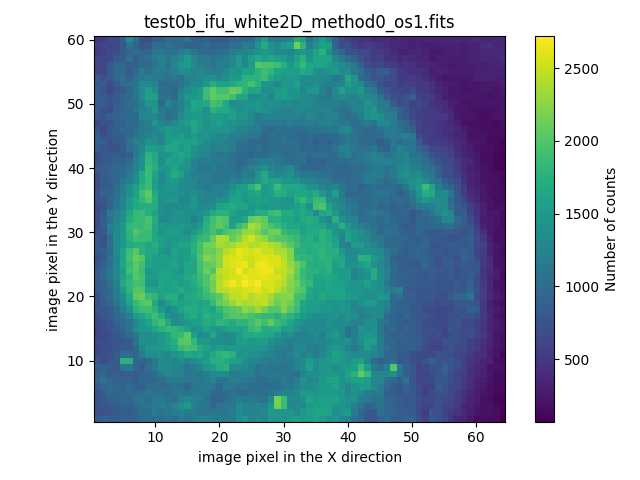
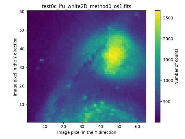
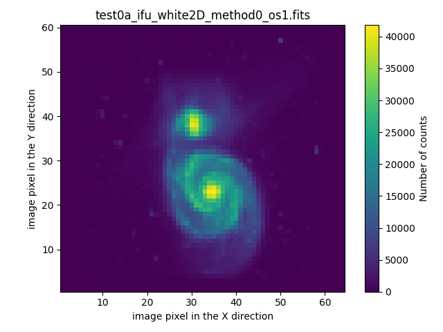
The files test0?_ifu_white2D_method0_os1.fits (with ? equal to a, b or c) can be examined with any visualization tool. The numina package provides the auxiliary script numina-ximshow for this purpose

(venv_frida) $ numina-ximshow \
test0?_ifu_white2D_method0_os1.fits \
--cmap viridis \
--cbar_orientation vertical \
--aspect equal \
--z1z2 minmax
../_images/test0a_2d.png ../_images/test0b_2d.png ../_images/test0c_2d.png

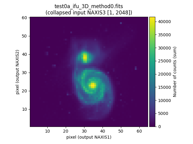
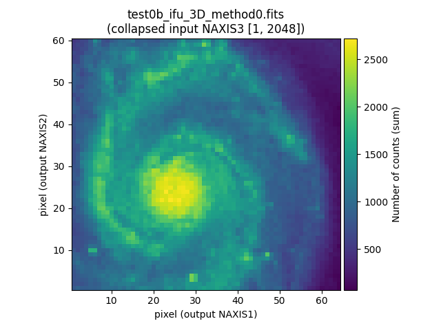
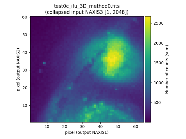
Note that it is also possible to visualize the collapsed view of the corresponding 3D data cubes, using in this case the numina script numina-extract_2d_slice_from_3d_cube (if no parameters are specified, it is assumed that the collapse is performed along NAXIS3 and all pixels in that direction are summed):

(venv_frida) $ numina-extract_2d_slice_from_3d_cube test0a_ifu_3D_method0.fits
(venv_frida) $ numina-extract_2d_slice_from_3d_cube test0b_ifu_3D_method0.fits
(venv_frida) $ numina-extract_2d_slice_from_3d_cube test0c_ifu_3D_method0.fits
../_images/test0a_3d_collapsed.png ../_images/test0b_3d_collapsed.png ../_images/test0c_3d_collapsed.png

Combination of individual exposures

The combination of the images is carried out using the numina script numina-generate_mosaic_of_2d_images, which takes as input an ASCII file containing the list of 2D FITS images to be combined, and the name of the output file.

The first step is then to generate an auxiliary text file with the names of the 2D FITS images to be combined.

(venv_frida) $ ls test0?_ifu_white2D_method0_os1.fits > list0_2d_images.txt
(venv_frida) $ cat list0_2d_images.txt
test0a_ifu_white2D_method0_os1.fits
test0b_ifu_white2D_method0_os1.fits
test0c_ifu_white2D_method0_os1.fits

To combine the 3 selected images, we only need to execute the numina script numina-generate_mosaic_of_2d_images:

(venv_frida) $ numina-generate_mosaic_of_2d_images \
  list0_2d_images.txt \
  combination_test0_2d.fits \
  --verbose
input_list: list0_2d_images.txt
output_filename: combination_test0_2d.fits
reproject_method: adaptive
extname_image: PRIMARY
extname_mask: None
combination_function: mean
output_3D_stack: None
verbose: True
echo: False

* Reading: test0a_ifu_white2D_method0_os1.fits
hdu2d_image.header['NAXIS1']=64
hdu2d_image.header['NAXIS2']=60
generating mask from np.nan values
Number of masked pixels / total: 0 / 3840

* Reading: test0b_ifu_white2D_method0_os1.fits
hdu2d_image.header['NAXIS1']=64
hdu2d_image.header['NAXIS2']=60
generating mask from np.nan values
Number of masked pixels / total: 0 / 3840

* Reading: test0c_ifu_white2D_method0_os1.fits
hdu2d_image.header['NAXIS1']=64
hdu2d_image.header['NAXIS2']=60
generating mask from np.nan values
Number of masked pixels / total: 0 / 3840
Total number of images to be combined: 3

wcs_mosaic2d=WCS Keywords

Number of WCS axes: 2
CTYPE : 'RA---TAN' 'DEC--TAN' 
CRVAL : 9.259258514947486e-06 0.0 
CRPIX : 125.16666693574936 120.50000000417663 
PC1_1 PC1_2  : 1.0 0.0 
PC2_1 PC2_2  : 0.0 1.0 
CDELT : -2.7777777777777233e-06 2.7777777777777233e-06 
NAXIS : 0  0
shape_mosaic2d=(240, 256)
Reprojection method: adaptive
Combination function: mean

Saving combined 2D image: combination_test0_2d.fits

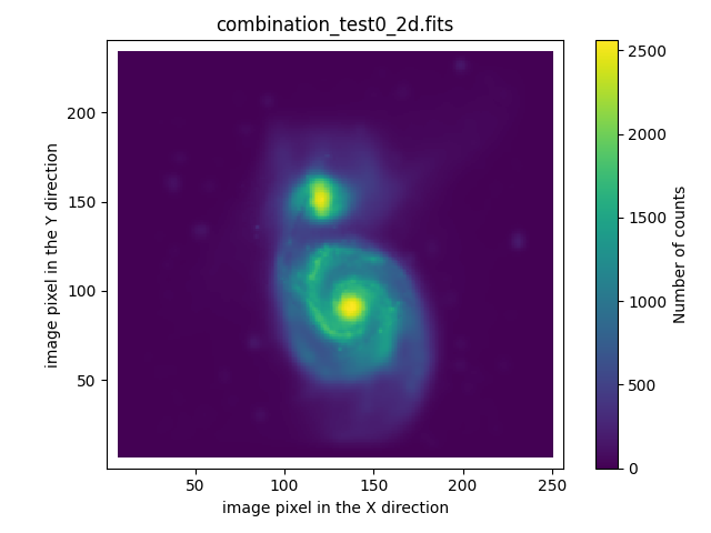
Next, we compare the result of the combination of the 3 simulated exposures with the first exposure alone: both cover the field of the coarse camera. The improvement in spatial resolution in the combined image is noticeable after including the two pointings made with the fine camera. Note that the combined image has the sampling corresponding to the fine camera. Hence, the number of counts shows such a different value in both images.

(venv_frida) $ numina-ximshow \
  combination_test0_2d.fits test0a_ifu_white2D_method0_os1.fits \
  --cmap viridis \
  --cbar_orientation vertical \
  --aspect equal \
  --z1z2 minmax
../_images/combined_test0_2d.png ../_images/single_test0a_2d.png

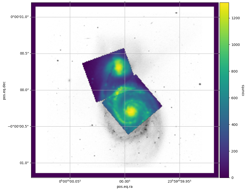
The following figure shows the result of combining the two exposures obtained with the ‘fine’ camera, represented on top of the first exposure calculated with an oversampling of 10 (file testa_ifu_white2D_method0_os10.fits).

../_images/combined_with_bw_background.png

Combination of 3D data cubes: example 1

We can start by combining the three 3D cubes generated in the previous section. Let us recall that in this case, the three cubes cover different solid angles on the celestial sphere but span the same wavelength range. Likewise, we do not have issues with differential atmospheric refraction within each data cube because we have assumed an airmass of 1.0.

The combination of the images is carried out using the numina script numina-generate_mosaic_of_3d_cubes, which takes as input an ASCII file containing the list of 3D FITS images to be combined, and the name of the output file.

(venv_frida) $ ls test0?_ifu_3D_method0.fits > list0_3d_cubes.txt
(venv_frida) $ cat list0_3d_cubes.txt
test0a_ifu_3D_method0.fits
test0b_ifu_3D_method0.fits
test0c_ifu_3D_method0.fits
(venv_frida) $ numina-generate_mosaic_of_3d_cubes \
 list0_3d_cubes.txt \
 all0_3d.fits \
 --reproject_method adaptive \
 --footprint \
 --verbose
input_list: list0_3d_cubes.txt
output_filename: all0_3d.fits
crval3out: None
cdelt3out: None
naxis3out: None
desired_celestial_2d_wcs: None
reproject_method: adaptive
parallel: False
extname_image: PRIMARY
output_celestial_2d_wcs: None
footprint: True
verbose: True
echo: False
Total number of images to be combined: 3
hdu.header["NAXIS1"]=64, hdu.header["NAXIS2"]=60, hdu.header["NAXIS3"]=2048

crval3out=<SpectralCoord 1.9344e-06 m>
cdelt3out=<Quantity 2.85e-10 m / pix>
naxis3out=2048
wavemax  =<Quantity 2.517795e-06 m>

wcs1d_spectral_mosaic=WCS Keywords

Number of WCS axes: 1
CTYPE : 'WAVE' 
CRVAL : 1.9344e-06 
CRPIX : 1.0 
PC1_1  : 1.0 
CDELT : 2.84999999999608e-10 
NAXIS : 2048  0

Celestial scales:
Image 1: 0.040 arcsec, 0.040 arcsec
Image 2: 0.010 arcsec, 0.010 arcsec
Image 3: 0.010 arcsec, 0.010 arcsec
Mosaic : 0.010 arcsec, 0.010 arcsec

wcs_mosaic2d=WCS Keywords

Number of WCS axes: 2
CTYPE : 'RA---TAN' 'DEC--TAN' 
CRVAL : 9.259258514947486e-06 0.0 
CRPIX : 125.16666693574936 120.50000000417663 
PC1_1 PC1_2  : 1.0 0.0 
PC2_1 PC2_2  : 0.0 1.0 
CDELT : -2.7777777777777233e-06 2.7777777777777233e-06 
NAXIS : 0  0

shape_mosaic2d=(240, 256)

NAXIS1, NAXIS2, NAXIS3 of 3D mosaic: 256, 240, 2048
Combined image will require 600.00 Mbyte

* Working with: test0a_ifu_3D_method0.fits
Old and new wavelength borders are the same.
-> Copying original data without spectral resampling.
Celestial WCS reprojection method: adaptive
Processing time for test0a_ifu_3D_method0.fits: 0:00:19.641678

* Working with: test0b_ifu_3D_method0.fits
Old and new wavelength borders are the same.
-> Copying original data without spectral resampling.
Celestial WCS reprojection method: adaptive
Processing time for test0b_ifu_3D_method0.fits: 0:00:02.132979

* Working with: test0c_ifu_3D_method0.fits
Old and new wavelength borders are the same.
-> Copying original data without spectral resampling.
Celestial WCS reprojection method: adaptive
Processing time for test0c_ifu_3D_method0.fits: 0:00:02.113682
Saving: all0_3d.fits

Total time: 0:00:24.587678
Done!

We can visualize the result using ds9:

(venv_frida) $ ds9 \
  -scale mode minmax \
  -geometry 1000x1000 \
  -wcs degrees \
  -multiframe \
  test0a_ifu_3D_method0.fits \
  test0b_ifu_3D_method0.fits \
  test0c_ifu_3D_method0.fits \
  all0_3d.fits \
  -lock slice image \
  -lock frame image \
  -zoom to fit \
  -cmap viridis \
  -match frame colorbar \
  -match frame wcs \
  -colorbar lock yes \
  -view multi yes
../_images/result_example1_with_ds9.png

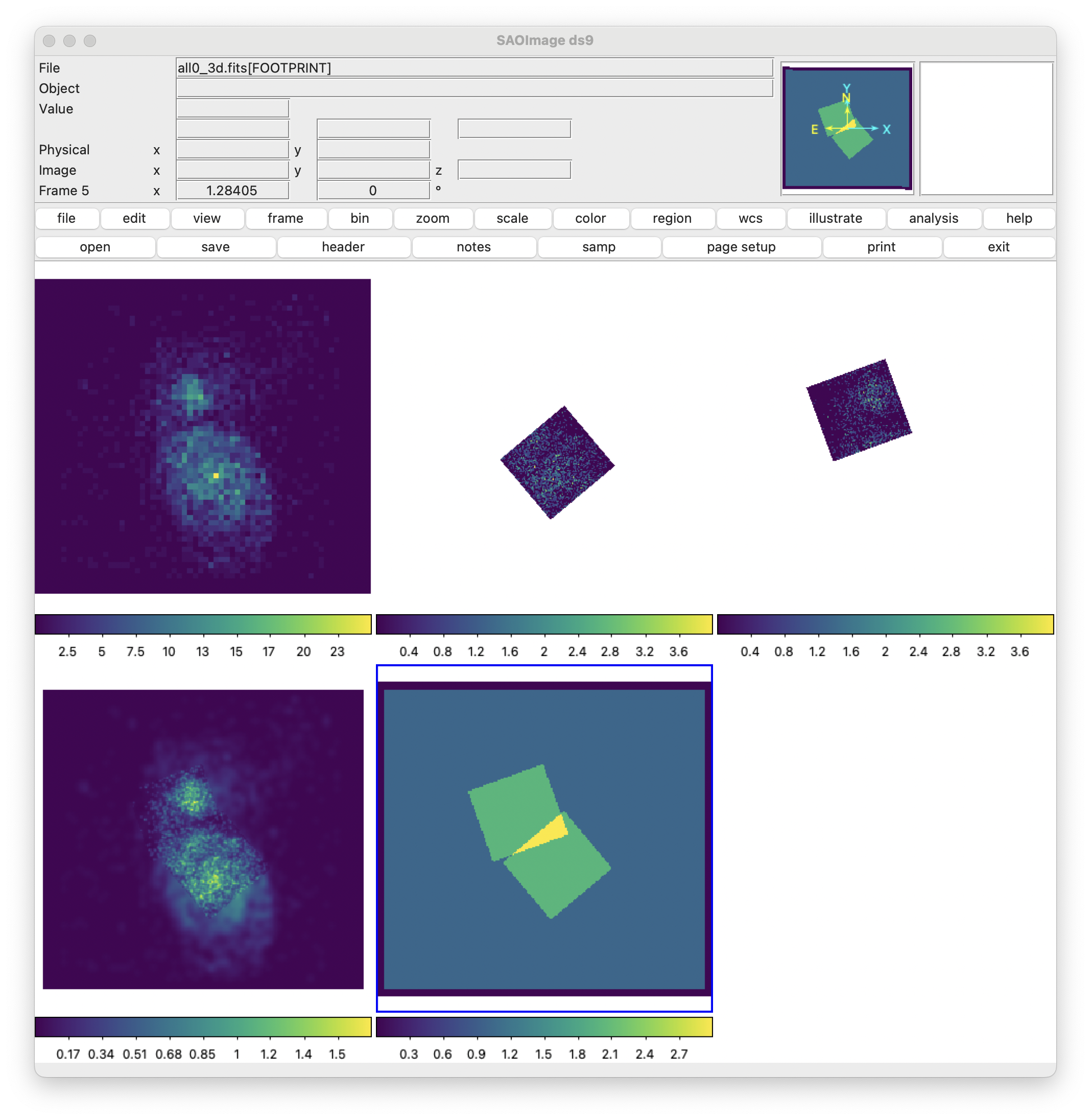
In the first row, the three individual exposures are shown. In the bottom row, the image on the left corresponds to the combination of the three individual exposures, while the image in the center is the footprint of that combination.

Combination of 3D data cubes: example 2

In this case, we will introduce the effect of differential atmospheric refraction, using exposures of the same region of the sky but with different airmasses and position angles.

Generation of individual exposures

For this example we are using the file scene_m51_3d.yaml.

Execute fridadrp-ifu_simulator:

(venv_frida) $ fridadrp-ifu_simulator \
  --scene scene_m51_3d.yaml \
  --grating medium-K \
  --scale fine \
  --airmass 1.0 \
  --parallactic_angle_deg 0 \
  --instrument_pa_deg 0 \
  --stop_after_ifu_3D_method0 \
  --prefix_intermediate_FITS test1a \
  --seed 1234
(venv_frida) $ fridadrp-ifu_simulator \
  --scene scene_m51_3d.yaml \
  --grating medium-K \
  --scale fine \
  --airmass 3.0 \
  --parallactic_angle_deg 45 \
  --instrument_pa_deg 20 \
  --stop_after_ifu_3D_method0 \
  --prefix_intermediate_FITS test1b \
  --seed 2345
(venv_frida) $ fridadrp-ifu_simulator \
  --scene scene_m51_3d.yaml \
  --grating medium-K \
  --scale fine \
  --airmass 3.0 \
  --parallactic_angle_deg -45 \
  --instrument_pa_deg 340 \
  --stop_after_ifu_3D_method0 \
  --prefix_intermediate_FITS test1c \
  --seed 3456

We have used again the parameter --stop_after_ifu_3D_method0 because we do not need to execute all the steps of the simulator to generate the images we will need in this example. In all cases, we are using the fine camera. In the first exposure, the airmass is 1.0. In the next two exposures we have chosen a high airmass to exaggerate the effect of atmospheric refraction, modifying both the value of the parallactic angle and the instrument.

Examining the individual data cubes before combining them

We can quickly visualize the result with the help of the ds9 program.

(venv_frida) $ ds9 \
-scale mode minmax \
-geometry 1000x1000 \
-wcs degrees \
-multiframe \
test1a_ifu_3D_method0.fits \
test1b_ifu_3D_method0.fits \
test1c_ifu_3D_method0.fits \
-lock slice image \
-lock frame image \
-zoom to fit \
-cmap viridis \
-match frame colorbar \
-colorbar lock yes \
-view multi yes
../_images/individual_3d_m51_exposures_with_ds9.png

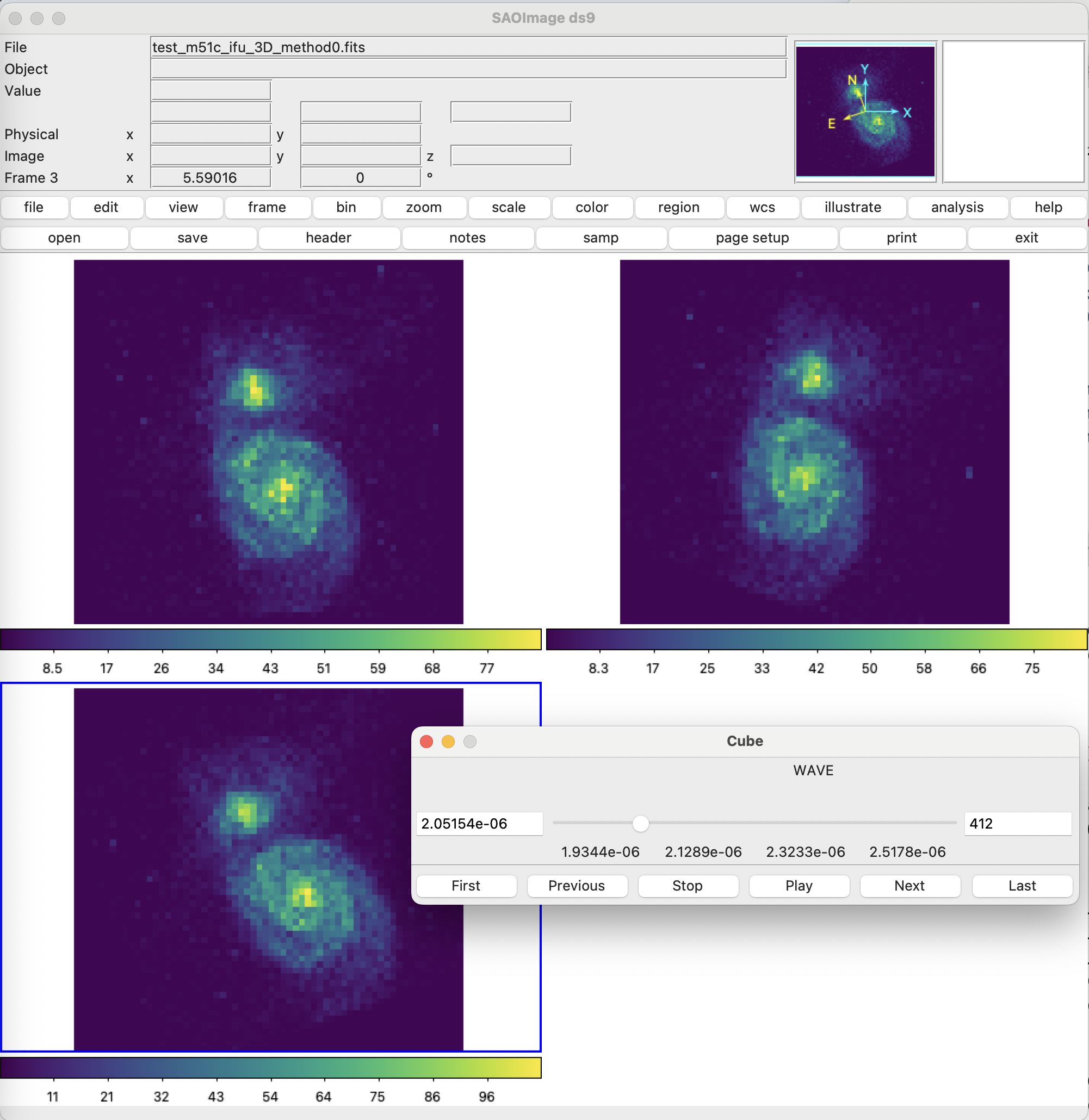
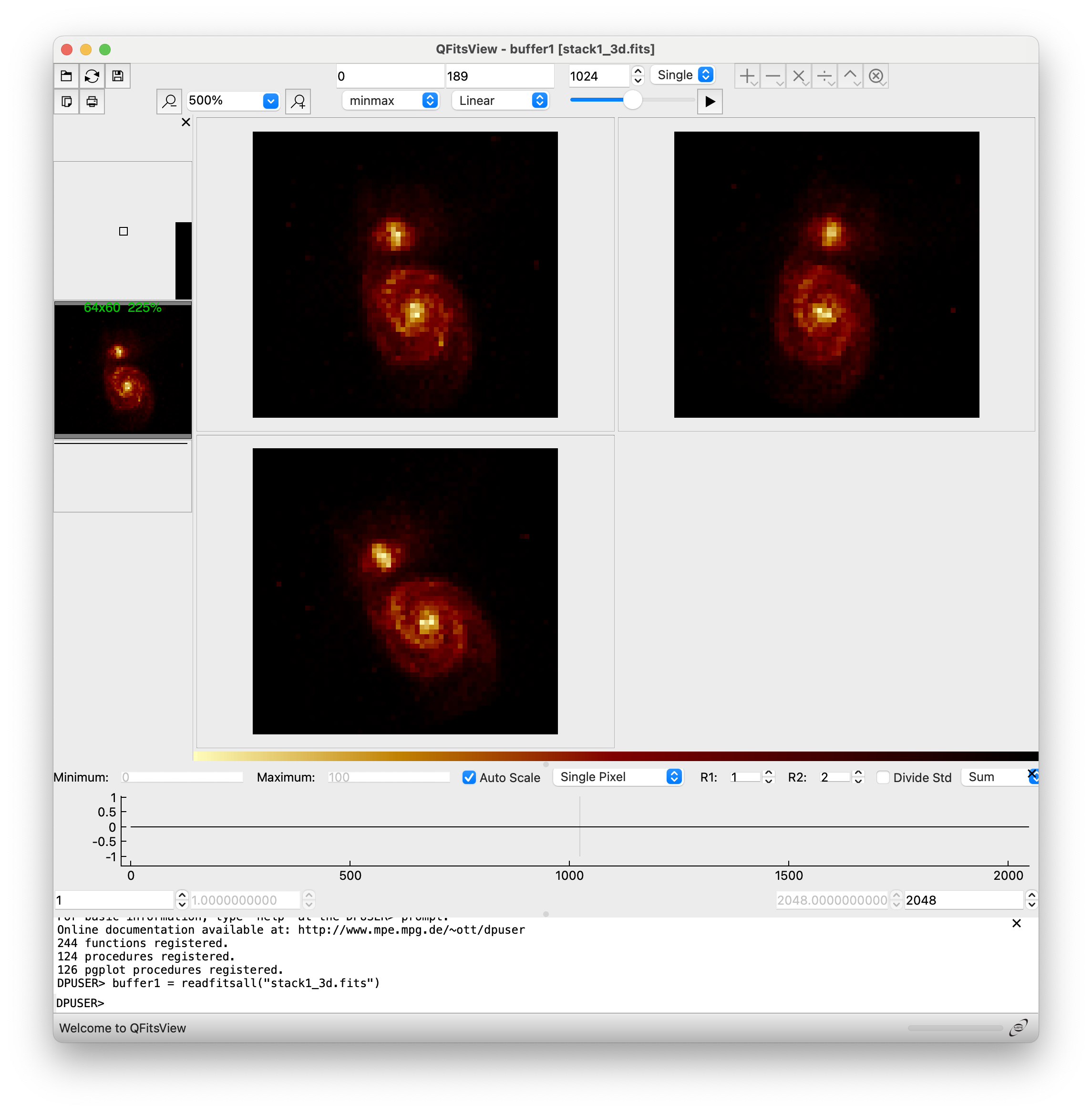
It is also possible to use qfitsview to visualize simultaneously the individual exposures. In this case, with the idea of being able to change the slice in the spectral direction simultaneously in the three exposures, we will first generate an auxiliary image that performs a stack of the HDUs (header and data units) from different FITS files into a single FITS file. For that purpose, we can employ the numina script numina-stack_hdus.

(venv_frida) $ fitsinfo test1*3D*.fits
Filename: test1a_ifu_3D_method0.fits
No.    Name      Ver    Type      Cards   Dimensions   Format
  0  PRIMARY       1 PrimaryHDU      82   (64, 60, 2048)   int16 (rescales to uint16)

Filename: test1b_ifu_3D_method0.fits
No.    Name      Ver    Type      Cards   Dimensions   Format
  0  PRIMARY       1 PrimaryHDU      84   (64, 60, 2048)   int16 (rescales to uint16)

Filename: test1c_ifu_3D_method0.fits
No.    Name      Ver    Type      Cards   Dimensions   Format
  0  PRIMARY       1 PrimaryHDU      84   (64, 60, 2048)   int16 (rescales to uint16)
(venv_frida) $ ls test1*3D*.fits > list1_3d_cubes.txt
(venv_frida) $ cat list1_3d_cubes.txt
test1a_ifu_3D_method0.fits
test1b_ifu_3D_method0.fits
test1c_ifu_3D_method0.fits
(venv_frida) $ numina-stack_hdus list1_3d_cubes.txt stack1_3d.fits
(venv_frida) $ qfitsview stack1_3d.fits

After executing the last command, select ‘Read All’ when qfitsview asks for the extension to read.

../_images/individual_3d_m51_exposures_with_qfitsview.png

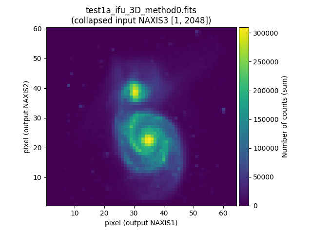
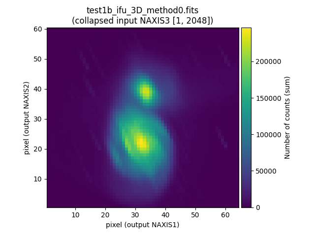
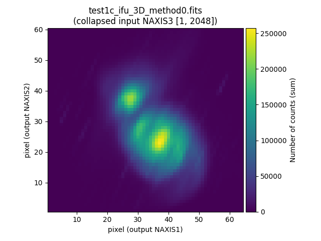
If we collapse the data cubes along the spectral direction (NAXIS3), the effect of atmospheric refraction is clearly noticeable.

(venv_frida) $ numina-extract_2d_slice_from_3d_cube test1a_ifu_3D_method0.fits
(venv_frida) $ numina-extract_2d_slice_from_3d_cube test1b_ifu_3D_method0.fits
(venv_frida) $ numina-extract_2d_slice_from_3d_cube test1c_ifu_3D_method0.fits
../_images/test1a_3d_collapsed.png ../_images/test1b_3d_collapsed.png ../_images/test1c_3d_collapsed.png

Combination of individual data cubes

If we combine the previous 3 data cubes ignoring the problem of atmospheric refraction, the result is not satisfactory.

(venv_frida) $ numina-generate_mosaic_of_3d_cubes \
  list1_3d_cubes.txt \
  combination_test1_3d.fits \
  --footprint \
  --verbose
input_list: list1_3d_cubes.txt
output_filename: combination_test1_3d.fits
crval3out: None
cdelt3out: None
naxis3out: None
desired_celestial_2d_wcs: None
reproject_method: adaptive
parallel: False
extname_image: PRIMARY
output_celestial_2d_wcs: None
footprint: True
verbose: True
echo: False
Total number of images to be combined: 3
hdu.header["NAXIS1"]=64, hdu.header["NAXIS2"]=60, hdu.header["NAXIS3"]=2048

crval3out=<SpectralCoord 1.9344e-06 m>
cdelt3out=<Quantity 2.85e-10 m / pix>
naxis3out=2048
wavemax  =<Quantity 2.517795e-06 m>

wcs1d_spectral_mosaic=WCS Keywords

Number of WCS axes: 1
CTYPE : 'WAVE' 
CRVAL : 1.9344e-06 
CRPIX : 1.0 
PC1_1  : 1.0 
CDELT : 2.84999999999608e-10 
NAXIS : 2048  0

Celestial scales:
Image 1: 0.010 arcsec, 0.010 arcsec
Image 2: 0.010 arcsec, 0.010 arcsec
Image 3: 0.010 arcsec, 0.010 arcsec
Mosaic : 0.010 arcsec, 0.010 arcsec

wcs_mosaic2d=WCS Keywords

Number of WCS axes: 2
CTYPE : 'RA---TAN' 'DEC--TAN' 
CRVAL : 4.296495291499103e-31 0.0 
CRPIX : 40.83076816991048 39.63542321434076 
PC1_1 PC1_2  : 1.0 0.0 
PC2_1 PC2_2  : 0.0 1.0 
CDELT : -2.7777777777777e-06 2.7777777777777e-06 
NAXIS : 0  0

shape_mosaic2d=(78, 81)

NAXIS1, NAXIS2, NAXIS3 of 3D mosaic: 81, 78, 2048
Combined image will require 61.70 Mbyte

* Working with: test1a_ifu_3D_method0.fits
Old and new wavelength borders are the same.
-> Copying original data without spectral resampling.
Celestial WCS reprojection method: adaptive
Processing time for test1a_ifu_3D_method0.fits: 0:00:00.577247

* Working with: test1b_ifu_3D_method0.fits
Old and new wavelength borders are the same.
-> Copying original data without spectral resampling.
Celestial WCS reprojection method: adaptive
Processing time for test1b_ifu_3D_method0.fits: 0:00:00.564567

* Working with: test1c_ifu_3D_method0.fits
Old and new wavelength borders are the same.
-> Copying original data without spectral resampling.
Celestial WCS reprojection method: adaptive
Processing time for test1c_ifu_3D_method0.fits: 0:00:00.568156
Saving: combination_test1_3d.fits

Total time: 0:00:01.816519
Done!
(venv_frida) $ fitsinfo combination_test1_3d.fits
Filename: combination_test1_3d.fits
No.    Name      Ver    Type      Cards   Dimensions   Format
  0  PRIMARY       1 PrimaryHDU      50   (81, 78, 2048)   float32
  1  FOOTPRINT     1 ImageHDU        29   (81, 78, 2048)   uint8
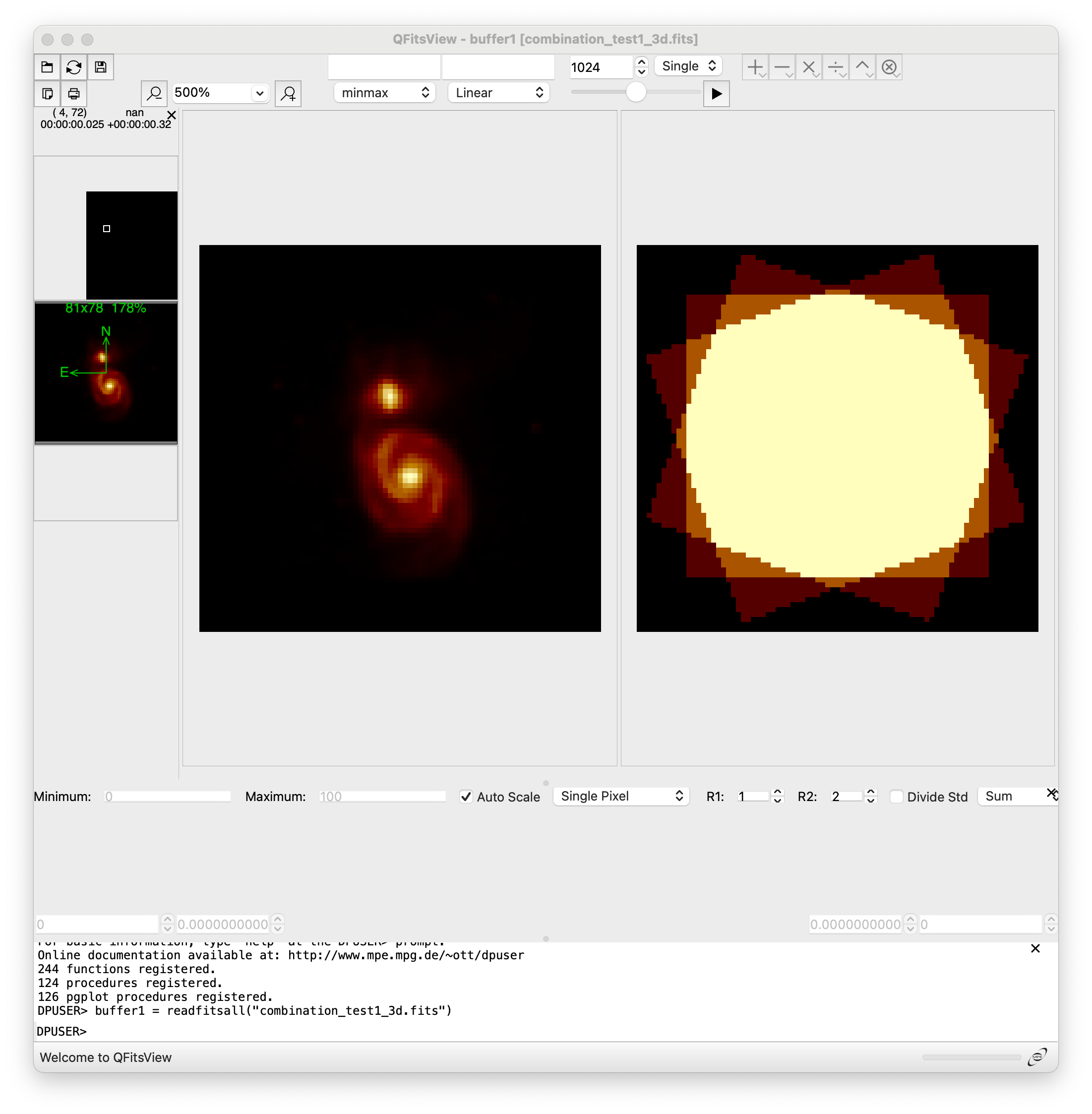
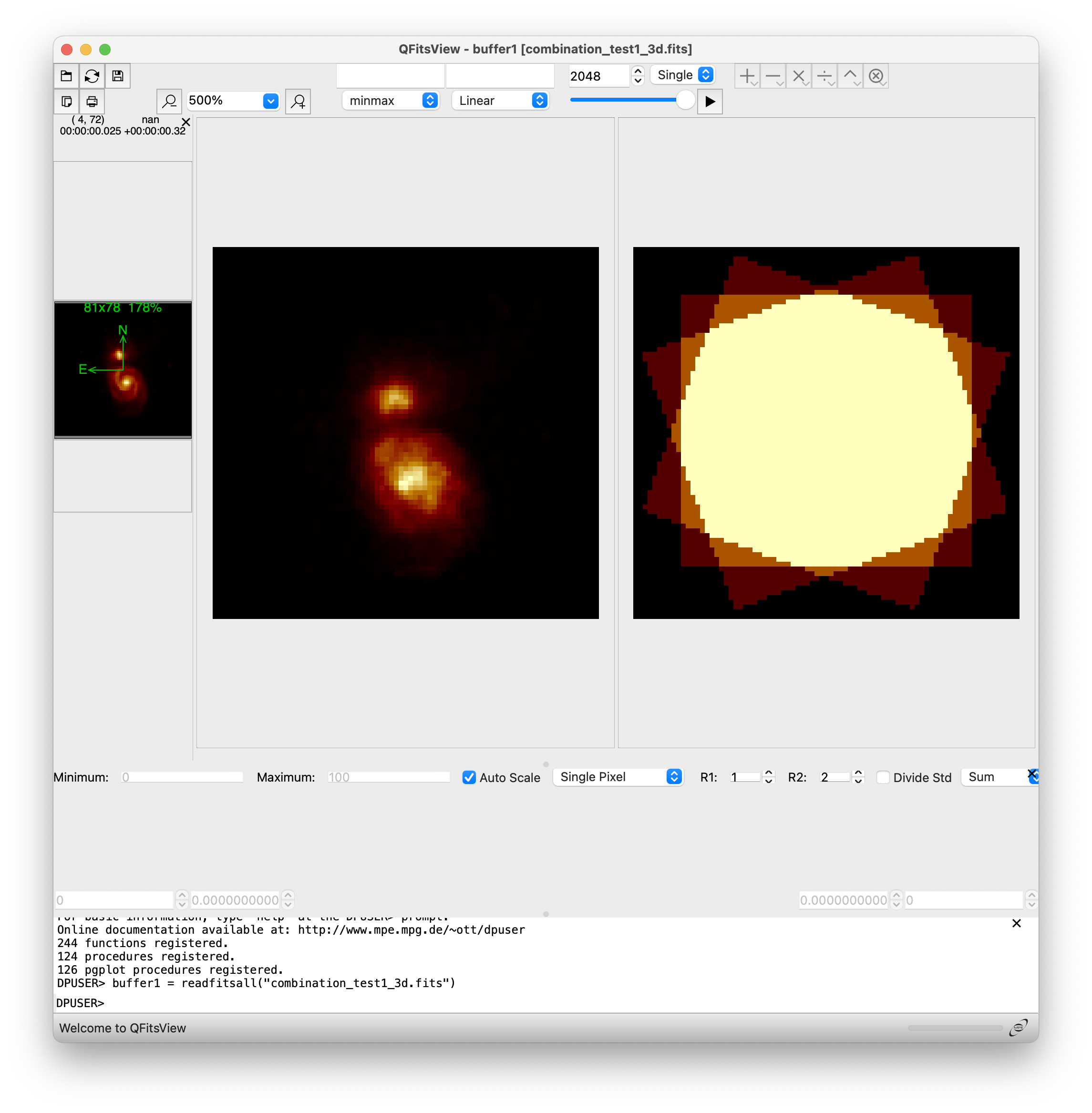
(venv_frida) $ qfitsview combination_test1_3d.fits

The initial spatial cut shown by qfitsview corresponds to pixel 1024 along NAXIS3. The corresponding image looks apparently normal.

../_images/combined_test1_3d_1024.png

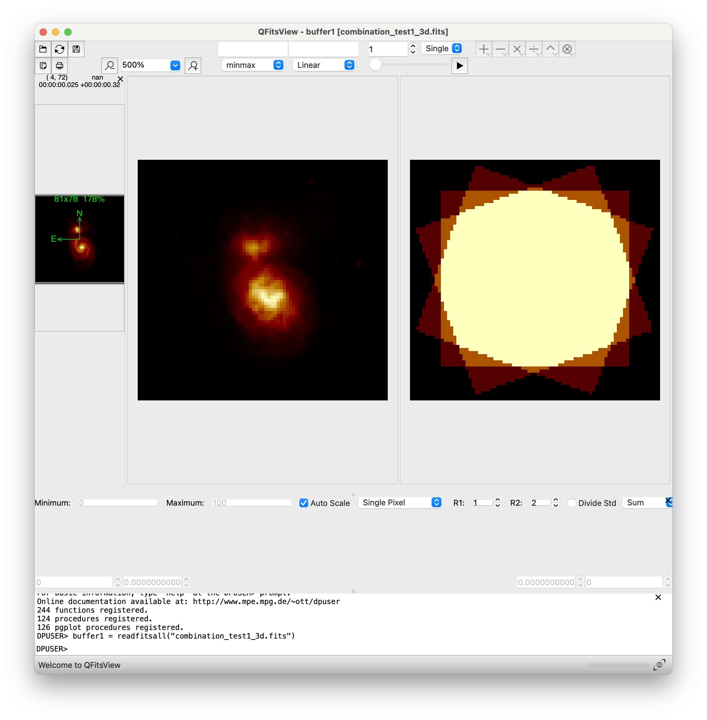
However, when we display the cut corresponding to pixel 1 or pixel 2048, the result is clearly not satisfactory.

../_images/combined_test1_3d_0001.png ../_images/combined_test1_3d_2048.png

Differencial atmospheric refraction correction

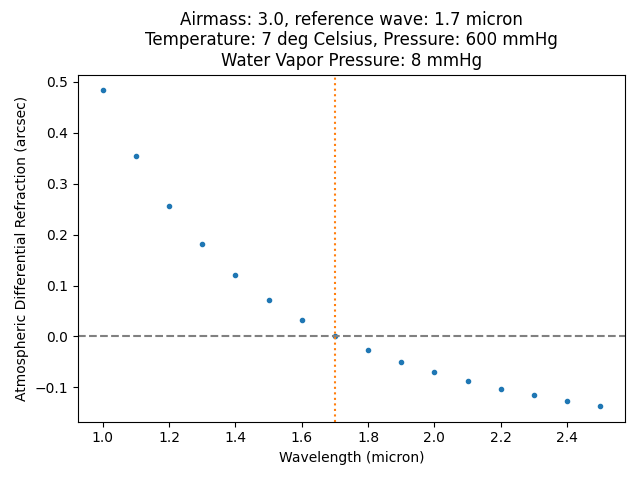
It is advisable to correct the individual exposures for differential atmospheric refraction (taking as reference the position of the image at the central wavelength along NAXIS3). To do this, we will start by using an auxiliary script that helps us visualize how significant the effect is in the images we are working with.

(venv_frida) $ numina-compute_adr_wavelength \
   --airmass 3 \
   --reference_wave_vacuum 1.7 \
   --wave_ini 1.0 \
   --wave_end 2.5 \
   --wave_step 0.1 \
   --wave_unit micron \
   --plots
Wavelength  ADR  
  micron   arcsec
---------- ------
     1.000  0.483
     1.100  0.355
     1.200  0.257
     1.300  0.181
     1.400  0.121
     1.500  0.072
     1.600  0.033
     1.700  0.000
     1.800 -0.027
     1.900 -0.051
     2.000 -0.071
     2.100 -0.088
     2.200 -0.102
     2.300 -0.115
     2.400 -0.127
     2.500 -0.137
../_images/adr_prediction.png

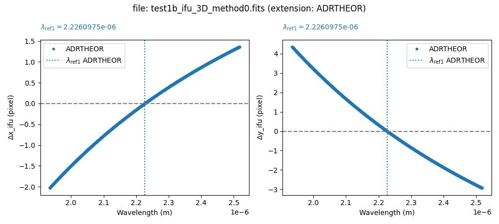
When correcting each individual exposure, we will first insert an extension with a binary table that stores the effect of atmospheric refraction into each FITS file.

(venv_frida) $ fitsheader -k airmass test1?_ifu_3D_method0.fits -f
         filename          AIRMASS
-------------------------- -------
test1a_ifu_3D_method0.fits     1.0
test1b_ifu_3D_method0.fits     3.0
test1c_ifu_3D_method0.fits     3.0

Only the second and third images need to be corrected. The first one was obtained with an airmass of 1.0.

(venv_frida) $ numina-include_adrtheor_in_3d_cube \
  test1b_ifu_3D_method0.fits \
  --verbose --plots
../_images/adr_test1b.png
(venv_frida) $ numina-include_adrtheor_in_3d_cube \
  test1c_ifu_3D_method0.fits \
  --verbose --plots
../_images/adr_test1c.png

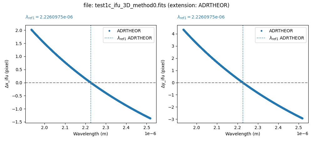
Important: the previous step stores the correction to be applied but does not apply it to the data. To perform this process, we need to use an additional script.

We see that a new extension ADRTHEOR has appeared in each data cube.

(venv_frida) $ fitsinfo test1*3D*.fits
Filename: test1a_ifu_3D_method0.fits
No.    Name      Ver    Type      Cards   Dimensions   Format
  0  PRIMARY       1 PrimaryHDU      82   (64, 60, 2048)   int16 (rescales to uint16)

Filename: test1b_ifu_3D_method0.fits
No.    Name      Ver    Type      Cards   Dimensions   Format
  0  PRIMARY       1 PrimaryHDU      84   (64, 60, 2048)   int16 (rescales to uint16)
  1  ADRTHEOR      1 BinTableHDU     21   2048R x 2C   [D, D]

Filename: test1c_ifu_3D_method0.fits
No.    Name      Ver    Type      Cards   Dimensions   Format
  0  PRIMARY       1 PrimaryHDU      84   (64, 60, 2048)   int16 (rescales to uint16)
  1  ADRTHEOR      1 BinTableHDU     21   2048R x 2C   [D, D]

We can also empirically measure atmospheric refraction in each data cube using cross-correlation.

(venv_frida) $ numina-measure_slice_xy_offsets_in_3d_cube \
  test1b_ifu_3D_method0.fits \
  100 \
  --iterate \
  --extname adrcross \
  --verbose --iterate --plots
(venv_frida) $ numina-measure_slice_xy_offsets_in_3d_cube \
  test1c_ifu_3D_method0.fits \
  100 \
  --iterate \
  --extname adrcross \
  --verbose --iterate --plots

The previous procedure has added a new extension ADRCROSS to each of the corrected images.

(venv_frida) $ fitsinfo test1*3D*.fits
Filename: test1a_ifu_3D_method0.fits
No.    Name      Ver    Type      Cards   Dimensions   Format
  0  PRIMARY       1 PrimaryHDU      82   (64, 60, 2048)   int16 (rescales to uint16)

Filename: test1b_ifu_3D_method0.fits
No.    Name      Ver    Type      Cards   Dimensions   Format
  0  PRIMARY       1 PrimaryHDU      84   (64, 60, 2048)   int16 (rescales to uint16)
  1  ADRTHEOR      1 BinTableHDU     21   2048R x 2C   [D, D]
  2  ADRCROSS      1 BinTableHDU     24   2048R x 2C   [D, D]

Filename: test1c_ifu_3D_method0.fits
No.    Name      Ver    Type      Cards   Dimensions   Format
  0  PRIMARY       1 PrimaryHDU      84   (64, 60, 2048)   int16 (rescales to uint16)
  1  ADRTHEOR      1 BinTableHDU     21   2048R x 2C   [D, D]
  2  ADRCROSS      1 BinTableHDU     24   2048R x 2C   [D, D]

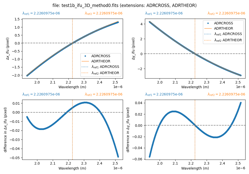
We can easily compare the expected atmospheric refraction with that calculated using the cross-correlation technique.

(venv_frida) $ numina-compare_adr_extensions_in_3d_cube \
  test1b_ifu_3D_method0.fits \
  adrcross adrtheor
../_images/adrcross_adrtheor.png

At this point, we can correct the exposures for atmospheric refraction using the preferred extension (in this case, ADRCROSS or ADRTHEOR).

(venv_frida) $ numina-adr_correction_from_extension_in_3d_cube \
  test1b_ifu_3D_method0.fits \
  --extname_adr adrtheor \
  --extname_mask None \
  --output test1b_ifu_3D_method0_corrected_ADRTHEOR.fits \
  --verbose
inputfile: test1b_ifu_3D_method0.fits
extname_adr: adrtheor
extname_mask: None
final_celestial_wcs: None
output: test1b_ifu_3D_method0_corrected_ADRTHEOR.fits
reproject_method: adaptive
verbose: True
echo: False
Filename: test1b_ifu_3D_method0.fits
No.    Name      Ver    Type      Cards   Dimensions   Format
  0  PRIMARY       1 PrimaryHDU      84   (64, 60, 2048)   int16 (rescales to uint16)   
  1  ADRTHEOR      1 BinTableHDU     21   2048R x 2C   [D, D]   
  2  ADRCROSS      1 BinTableHDU     24   2048R x 2C   [D, D]   
None
Reading ADR correction from ADRTHEOR extension
Generating mask from np.nan in PRIMARY HDU
Number of masked pixels in the input 3D array: 0
Center IFU coord: <SkyCoord (ICRS): (ra, dec) in deg
    (4.29649529e-31, 0.)>

wcs2d_blue:
WCS Keywords

Number of WCS axes: 2
CTYPE : 'RA---TAN' 'DEC--TAN' 
CRVAL : 0.0 0.0 
CRPIX : 30.47089355891503 34.85143279557968 
CD1_1 CD1_2  : -2.6102572799608e-06 9.5005595368241e-07 
CD2_1 CD2_2  : 9.5005595368241e-07 2.6102572799608e-06 
NAXIS : 64  60

wcs2d_red:
WCS Keywords

Number of WCS axes: 2
CTYPE : 'RA---TAN' 'DEC--TAN' 
CRVAL : 0.0 0.0 
CRPIX : 33.86438885042125 27.574058674345103 
CD1_1 CD1_2  : -2.6102572799608e-06 9.5005595368241e-07 
CD2_1 CD2_2  : 9.5005595368241e-07 2.6102572799608e-06 
NAXIS : 64  60

wcs_mosaic2d:
WCS Keywords

Number of WCS axes: 2
CTYPE : 'RA---TAN' 'DEC--TAN' 
CRVAL : 4.296495291499103e-31 0.0 
CRPIX : 43.11360516821077 43.03043722644195 
PC1_1 PC1_2  : 1.0 0.0 
PC2_1 PC2_2  : 0.0 1.0 
CDELT : -2.7777777777777233e-06 2.7777777777777233e-06 
NAXIS : 0  0
shape_mosaic2d: (84, 86)
NAXIS1, NAXIS2, NAXIS3 of corrected 3D cube: 86, 84, 2048
Reprojection method: adaptive (please wait...)
Reprojection finished! (elapsed time: 13.683667 seconds)

Flux check:
- total counts in original  3D cube: 84579025
- total counts in corrected 3D cube: 84272326.60160962
- ratio original/corrected.........: 1.003639372623949

Footprint coverage (fraction): 0.4813108729365656

header3d_corrected:
WCSAXES =                    3 / Number of coordinate axes                      
CRPIX1  =      43.113605168211 / Pixel coordinate of reference point            
CRPIX2  =      43.030437226442 / Pixel coordinate of reference point            
CRPIX3  =                  1.0 / Pixel coordinate of reference point            
CDELT1  = -2.7777777777777E-06 / [deg] Coordinate increment at reference point  
CDELT2  =  2.7777777777777E-06 / [deg] Coordinate increment at reference point  
CDELT3  = 2.85000000000032E-10 / [m] Coordinate increment at reference point    
CUNIT1  = 'deg'                / Units of coordinate increment and value        
CUNIT2  = 'deg'                / Units of coordinate increment and value        
CUNIT3  = 'm       '           / Units of coordinate increment and value        
CTYPE1  = 'RA---TAN'           / Right ascension, gnomonic projection           
CTYPE2  = 'DEC--TAN'           / Declination, gnomonic projection               
CTYPE3  = 'WAVE    '           / Vacuum wavelength (linear)                     
CRVAL1  =  4.2964952914991E-31 / [deg] Coordinate value at reference point      
CRVAL2  =                  0.0 / [deg] Coordinate value at reference point      
CRVAL3  =           1.9344E-06 / [m] Coordinate value at reference point        
LONPOLE =                180.0 / [deg] Native longitude of celestial pole       
LATPOLE =                  0.0 / [deg] Native latitude of celestial pole        
MJDREF  =                  0.0 / [d] MJD of fiducial time                       
RADESYS = 'ICRS'               / Equatorial coordinate system                   

Saving file: test1b_ifu_3D_method0_corrected_ADRTHEOR.fits
(venv_frida) $ numina-adr_correction_from_extension_in_3d_cube \
  test1c_ifu_3D_method0.fits \
  --extname_adr adrtheor \
  --extname_mask None \
  --output test1c_ifu_3D_method0_corrected_ADRTHEOR.fits \
  --verbose
inputfile: test1c_ifu_3D_method0.fits
extname_adr: adrtheor
extname_mask: None
final_celestial_wcs: None
output: test1c_ifu_3D_method0_corrected_ADRTHEOR.fits
reproject_method: adaptive
verbose: True
echo: False
Filename: test1c_ifu_3D_method0.fits
No.    Name      Ver    Type      Cards   Dimensions   Format
  0  PRIMARY       1 PrimaryHDU      84   (64, 60, 2048)   int16 (rescales to uint16)   
  1  ADRTHEOR      1 BinTableHDU     21   2048R x 2C   [D, D]   
  2  ADRCROSS      1 BinTableHDU     24   2048R x 2C   [D, D]   
None
Reading ADR correction from ADRTHEOR extension
Generating mask from np.nan in PRIMARY HDU
Number of masked pixels in the input 3D array: 0
Center IFU coord: <SkyCoord (ICRS): (ra, dec) in deg
    (4.29649529e-31, 0.)>

wcs2d_blue:
WCS Keywords

Number of WCS axes: 2
CTYPE : 'RA---TAN' 'DEC--TAN' 
CRVAL : 0.0 0.0 
CRPIX : 34.52910644625764 34.8514327982211 
CD1_1 CD1_2  : -2.6102572799608e-06 -9.5005595368241e-07 
CD2_1 CD2_2  : -9.5005595368241e-07 2.6102572799608e-06 
NAXIS : 64  60

wcs2d_red:
WCS Keywords

Number of WCS axes: 2
CTYPE : 'RA---TAN' 'DEC--TAN' 
CRVAL : 0.0 0.0 
CRPIX : 31.135611152816494 27.574058672835317 
CD1_1 CD1_2  : -2.6102572799608e-06 -9.5005595368241e-07 
CD2_1 CD2_2  : -9.5005595368241e-07 2.6102572799608e-06 
NAXIS : 64  60

wcs_mosaic2d:
WCS Keywords

Number of WCS axes: 2
CTYPE : 'RA---TAN' 'DEC--TAN' 
CRVAL : 4.296495291499103e-31 0.0 
CRPIX : 44.22578218603953 43.03043723461774 
PC1_1 PC1_2  : 1.0 0.0 
PC2_1 PC2_2  : 0.0 1.0 
CDELT : -2.7777777777777233e-06 2.7777777777777233e-06 
NAXIS : 0  0
shape_mosaic2d: (84, 86)
NAXIS1, NAXIS2, NAXIS3 of corrected 3D cube: 86, 84, 2048
Reprojection method: adaptive (please wait...)
Reprojection finished! (elapsed time: 13.578309 seconds)

Flux check:
- total counts in original  3D cube: 84480108
- total counts in corrected 3D cube: 84274917.53627832
- ratio original/corrected.........: 1.0024347750163427

Footprint coverage (fraction): 0.4813119544011282

header3d_corrected:
WCSAXES =                    3 / Number of coordinate axes                      
CRPIX1  =       44.22578218604 / Pixel coordinate of reference point            
CRPIX2  =      43.030437234618 / Pixel coordinate of reference point            
CRPIX3  =                  1.0 / Pixel coordinate of reference point            
CDELT1  = -2.7777777777777E-06 / [deg] Coordinate increment at reference point  
CDELT2  =  2.7777777777777E-06 / [deg] Coordinate increment at reference point  
CDELT3  = 2.85000000000032E-10 / [m] Coordinate increment at reference point    
CUNIT1  = 'deg'                / Units of coordinate increment and value        
CUNIT2  = 'deg'                / Units of coordinate increment and value        
CUNIT3  = 'm       '           / Units of coordinate increment and value        
CTYPE1  = 'RA---TAN'           / Right ascension, gnomonic projection           
CTYPE2  = 'DEC--TAN'           / Declination, gnomonic projection               
CTYPE3  = 'WAVE    '           / Vacuum wavelength (linear)                     
CRVAL1  =  4.2964952914991E-31 / [deg] Coordinate value at reference point      
CRVAL2  =                  0.0 / [deg] Coordinate value at reference point      
CRVAL3  =           1.9344E-06 / [m] Coordinate value at reference point        
LONPOLE =                180.0 / [deg] Native longitude of celestial pole       
LATPOLE =                  0.0 / [deg] Native latitude of celestial pole        
MJDREF  =                  0.0 / [d] MJD of fiducial time                       
RADESYS = 'ICRS'               / Equatorial coordinate system                   

Saving file: test1c_ifu_3D_method0_corrected_ADRTHEOR.fits

Next, we add the 3 cubes (the first one uncorrected and the second and third cubes corrected).

(venv_frida) $ ls test1a_ifu_3D_method0.fits \
  test1*_ADRTHEOR.fits > list1_3d_images_ADRTHEOR.txt
(venv_frida) $ cat list1_3d_images_ADRTHEOR.txt
test1a_ifu_3D_method0.fits
test1b_ifu_3D_method0_corrected_ADRTHEOR.fits
test1c_ifu_3D_method0_corrected_ADRTHEOR.fits
(venv_frida) $ numina-generate_mosaic_of_3d_cubes \
  list1_3d_images_ADRTHEOR.txt \
  combination_test1_3d_ADRTHEOR.fits \
  --verbose
input_list: list1_3d_images_ADRTHEOR.txt
output_filename: combination_test1_3d_ADRTHEOR.fits
crval3out: None
cdelt3out: None
naxis3out: None
desired_celestial_2d_wcs: None
reproject_method: adaptive
parallel: False
extname_image: PRIMARY
output_celestial_2d_wcs: None
footprint: True
verbose: True
echo: False
Total number of images to be combined: 3
hdu.header["NAXIS1"]=64, hdu.header["NAXIS2"]=60, hdu.header["NAXIS3"]=2048
hdu.header["NAXIS1"]=86, hdu.header["NAXIS2"]=84, hdu.header["NAXIS3"]=2048

crval3out=<SpectralCoord 1.9344e-06 m>
cdelt3out=<Quantity 2.85e-10 m / pix>
naxis3out=2048
wavemax  =<Quantity 2.517795e-06 m>

wcs1d_spectral_mosaic=WCS Keywords

Number of WCS axes: 1
CTYPE : 'WAVE' 
CRVAL : 1.9344e-06 
CRPIX : 1.0 
PC1_1  : 1.0 
CDELT : 2.84999999999608e-10 
NAXIS : 2048  0

Celestial scales:
Image 1: 0.010 arcsec, 0.010 arcsec
Image 2: 0.010 arcsec, 0.010 arcsec
Image 3: 0.010 arcsec, 0.010 arcsec
Mosaic : 0.010 arcsec, 0.010 arcsec

wcs_mosaic2d=WCS Keywords

Number of WCS axes: 2
CTYPE : 'RA---TAN' 'DEC--TAN' 
CRVAL : 7.160825485831836e-31 0.0 
CRPIX : 44.22578218656925 43.03043723364317 
PC1_1 PC1_2  : 1.0 0.0 
PC2_1 PC2_2  : 0.0 1.0 
CDELT : -2.7777777777777e-06 2.7777777777777e-06 
NAXIS : 0  0

shape_mosaic2d=(84, 87)

NAXIS1, NAXIS2, NAXIS3 of 3D mosaic: 87, 84, 2048
Combined image will require 71.37 Mbyte

* Working with: test1a_ifu_3D_method0.fits
Old and new wavelength borders are the same.
-> Copying original data without spectral resampling.
Celestial WCS reprojection method: adaptive
Processing time for test1a_ifu_3D_method0.fits: 0:00:00.736472

* Working with: test1b_ifu_3D_method0_corrected_ADRTHEOR.fits
Old and new wavelength borders are the same.
-> Copying original data without spectral resampling.
Celestial WCS reprojection method: adaptive
Processing time for test1b_ifu_3D_method0_corrected_ADRTHEOR.fits: 0:00:01.206074

* Working with: test1c_ifu_3D_method0_corrected_ADRTHEOR.fits
Old and new wavelength borders are the same.
-> Copying original data without spectral resampling.
Celestial WCS reprojection method: adaptive
Processing time for test1c_ifu_3D_method0_corrected_ADRTHEOR.fits: 0:00:01.385879
Saving: combination_test1_3d_ADRTHEOR.fits

Total time: 0:00:03.422615
Done!
(venv_frida) $ ds9 \
  -scale mode minmax \
  -geometry 1000x1000 \
  -wcs degrees \
  -multiframe \
  test1a_ifu_3D_method0.fits \
  test1b_ifu_3D_method0_corrected_ADRTHEOR.fits \
  test1c_ifu_3D_method0_corrected_ADRTHEOR.fits \
  combination_test1_3d_ADRTHEOR.fits \
  -lock slice image \
  -lock frame image \
  -zoom to fit \
  -cmap viridis \
  -match frame colorbar \
  -match frame wcs \
  -colorbar lock yes \
  -view multi yes
../_images/result_example1_ADRTHEOR_with_ds9.png

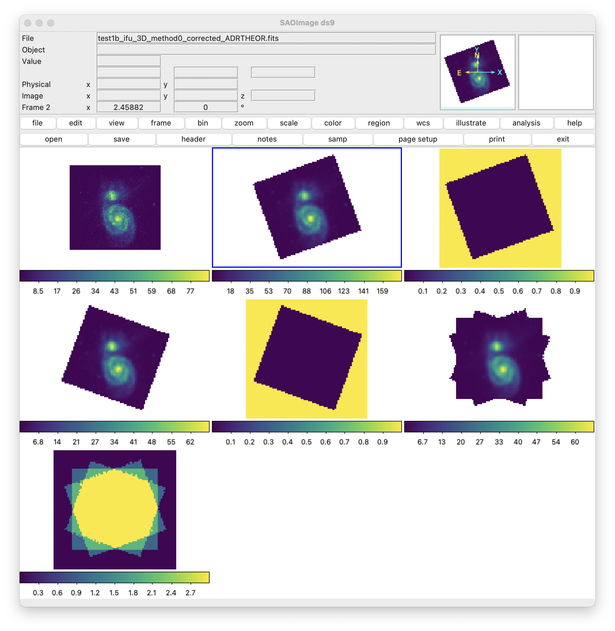
In the upper image, from top to bottom and left to right, we have the cubes corresponding to: the first exposure, the second exposure corrected using ADRTHEOR, the mask of the previous cube, the third exposure corrected using ADRTHEOR, the mask of the previous cube, the combination of the 3 cubes, and the footprint of that combination. It is very interesting to move along the wavelength using the slider that ds9 provides in an auxiliary window.

Finally, we can compare the effect of correcting or not correcting for atmospheric refraction.

(venv_frida) $ ds9 \
  -scale mode minmax \
  -geometry 1000x1000 \
  -wcs degrees \
  -multiframe \
  combination_test1_3d.fits \
  combination_test1_3d_ADRTHEOR.fits \
  -lock slice image \
  -lock frame image \
  -zoom to fit \
  -cmap viridis \
  -match frame colorbar \
  -match frame wcs \
  -colorbar lock yes \
  -view multi yes
../_images/result_example1_without_with_ADR_ds9.png

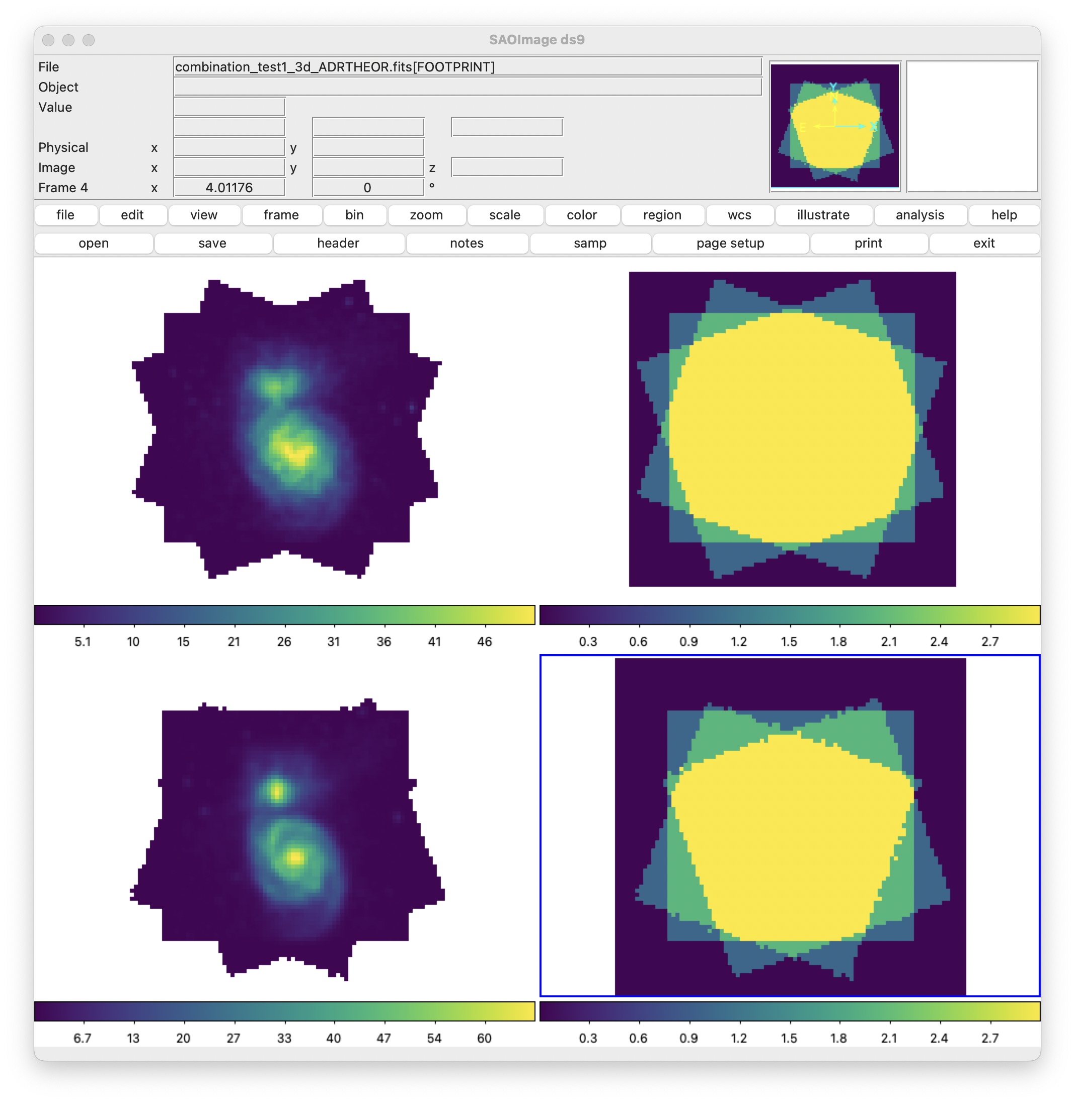
The top row shows the combined cube and the associated footprint when the combination is carried out without taking into account the effect of differential atmospheric refraction, while the bottom row shows the result when this effect is taken into account. Once again, it is important to interact with the display by moving along the wavelength.

ToDo: add the option to correct for atmospheric refraction by generating a corrected cube with a predefined celestial WCS with an arbitrary size. In this way, instead of interpolating when correcting for atmospheric refraction and when combining cubes with different pointings, we would only perform a single interpolation at the time of atmospheric refraction correction.