MEGARA Tools
In this section we describe a series of software tools that have been developed by the MEGARA team and that can be used to visualize and analyze the products of the MEGARA DRP. The first two tools (visualization and cube) are already included as part of the MEGARA DRP distribution. The rest conform their own software package megara-tools, which is also available through GitHub at https://github.com/guaix-ucm/megara-tools. The installation requires to follow one of these three strategies:
To install the latest stable version:
(megara) $ pip install megara-tools[hypercube]

# Note: mac OS under zsh should use:
# $ pip install "megara-tools[hypercube]"
or, if you do not want hypercube to be installed (as it includes pysynphot as a dependency, which is no longer actively developed), simply do:
(megara) $ pip install megara-tools
To install the development version:
(megara) $ pip install git+https://github.com/guaix-ucm/megara-tools.git
To develop your own tools based on megara-tools:
(megara) $ git clone https://github.com/guaix-ucm/megara-tools.git
(megara) $ cd megara-tools
(megara) $ pip install -e .
All tools described in this section should be under Python >=3.5 and
should be run within the MEGARA DRP environment. For all tools besides
megaratools-cube and megaratools-hypercube, these can be run under
the megaradrp Python package (numina and megaradrp versions 0.21+
and 0.9+, respectively) or under the development version. For
megaratools-cube and megaratools-hypercube, the development version
or Python packages with release date after July 1st 2020
(numina and megaradrp versions 0.22+ and 0.10+, respectively) should
be used. All these tools have been extensively tested in Mac OS X (10.10
to 10.15) and linux machines. Some of the examples below make use of
test/* folder data that are downloaded when executing the code tests.
Downloading sample data
The sample data employed in this section is available at this link: test-megaratools_v1.tar.gz
If you find any trouble trying to download the previous file, try with the following command line:
(megara) $ curl -O https://guaix.fis.ucm.es/data/megaradrp/test-megaratools_v1.tar.gz
After decompressing and extracting the contents of this file, you should
generate a subdirectory test/ with all the sample files required in the
following examples.
Megaradrp.Visualization
As part of the MEGARA DRP we also provide a tool to visualize the RSS
frames generated when processing LCB IFU data. This tool is best suited
for visualizing final_rss.fits RSS images (or, equivalently,
reduced_rss.fits images) obtained after running the MegaraLcbImage
processing recipe. The way to execute this code is to use the following
command under the corresponding MEGARA environment:
(megara) $ python -m megaradrp.visualization \
           test/final_rss_M32_MR-G.fits --label "flux (Jy)" --wcs-grid
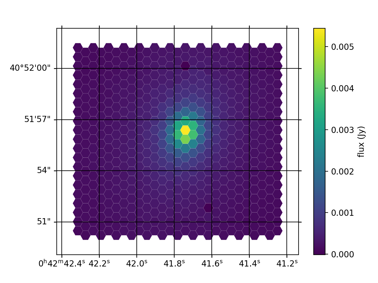
Figure 17: Example of reconstructed final_rss.fits (sky subtracted, wavelength and flux calibrated) image of the center of Local Group galaxy M32 in the MR-G setup. This image is generated using the megaradrp.visualization code included in the MEGARA DRP distribution.
(megara) $ python -m megaradrp.visualization \
           test/final_rss_M15_HR-R.fits --label "flux (Jy)" --wcs-grid
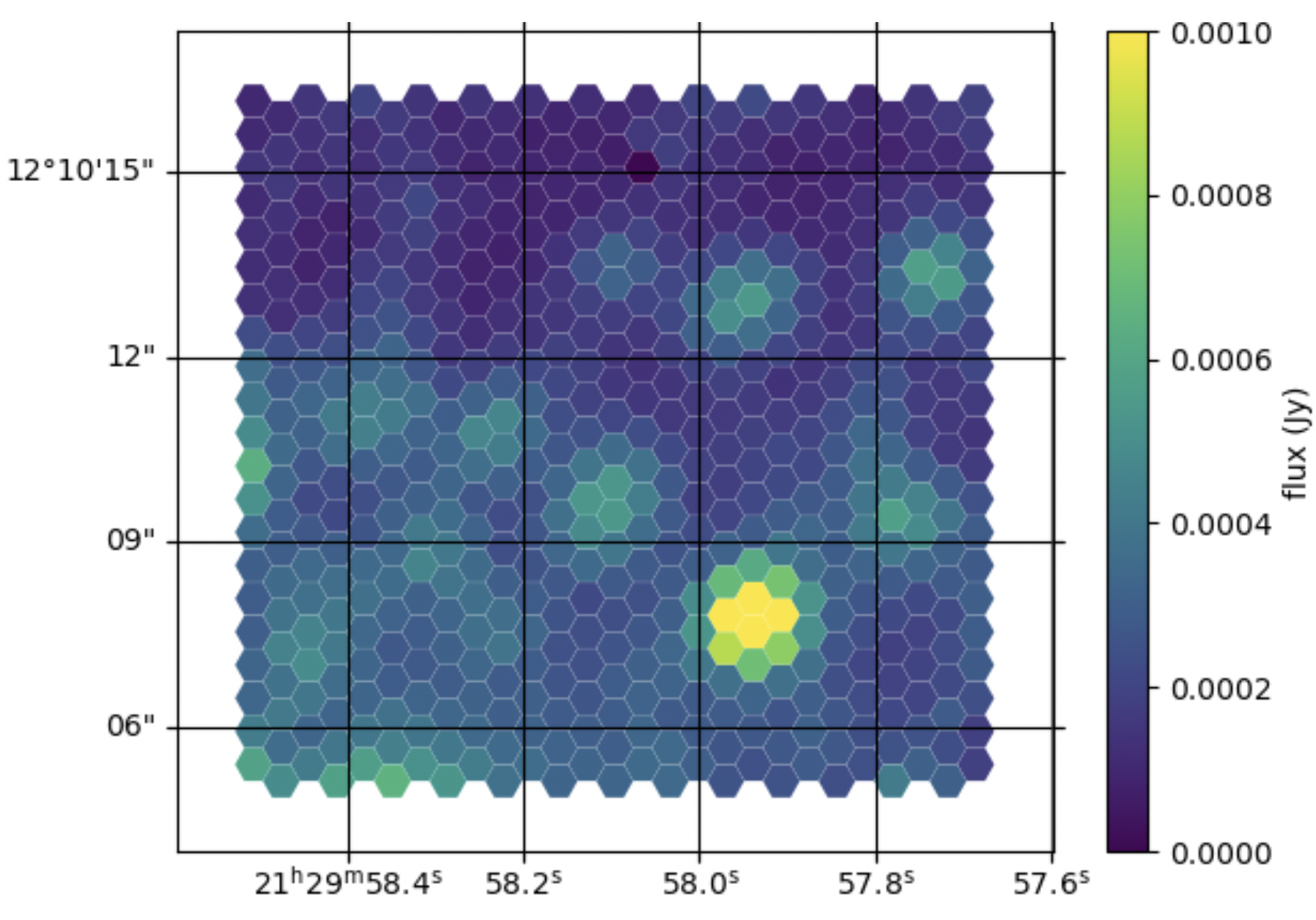
Figure 18: Example of reconstructed final_rss.fits (sky subtracted, wavelength and flux calibrated) image of the center of globular cluster M15 in the HR-R setup. This image is generated using the megaradrp-visualization code included in the MEGARA DRP distribution.
Figures 17 and 18 show two examples of the output generated by this code for commissioning observations of Local Group galaxy M32 and Galactic Globular Cluster M15, respectively.
As for the other commands, adding the -h flag would provide the help and syntax for using this command. The result is the following:
(megara) $ python -m megaradrp.visualization --help
Note that this visualization tool can be also used to display output RSS
files from the analyze_rss.py tool described below. As an example, the
command to display the flux the first of the two gaussians fit to a
specific emission line analyzed with that code would be (see Section
6.8):
(megara) $ python -m megaradrp.visualization \
           test/analyze_rss_Halpha.fits -c 22 --min-cut 10. --max-cut 400.
Megaradrp-Cube
This tool allows to conver the output RSS file from the MegaraLcbImage recipe (with or without the sky spectrum subtracted) into a FITS datacube (x,y,z) where the z axis corresponds to every lambda in the input RSS file and the (x,y) axes correspond to the two coordinates in the sky (RA & Dec if instrument PA is 0º). Since this tool is now part of the MEGARA DRP it should be run from within the DRP environment by doing:
(megara) $ megaradrp-cube -h
Default parameters for the --disable-scaling and --wcs-pa-from-header
options should be fine for regular MEGARA data processed with the DRP.
An alternative software with similar scope has been developed by Javier Zaragoza Cardiel (from INAOE) and can be obtained through GitHub at https://github.com/javierzaragoza/megararss2cube.
Extract spectrum: megaratools-extract_spectrum
This tool is the first being described in this cookbook that is part of the megaratools package available through GitHub at https://github.com/guaix-ucm/megara-tools. The objective of this tool is to generate an extracted (1D) spectrum of a given fiber or set of fibers. The main parameter determining the fiber(s) to be extracted is the fiber number as measured in the pseudo-slit (from 1 to 623 in the case of the LCB; 1 to 644 for the MOS). Since the RSS products of the MegaraMosImage recipe already include an extension with the 7 fibers of the each minibundle added together, this is particularly useful for extracting spectra of different regions from processed LCB RSS frames. The resulting extracted spectrum shares wavelength calibration solution with the RSS. All tools included in the megaratools package can be called as an argument for the Python main interpreter or as executables on their own, although the latter option is recommended:
(megara) $ megaratools-extract_spectrum -h
The result of the task when called using the help (-h) argument is:
The table with the fiber ids (-t) is a simple ASCII file in which one of
the (space-separated) columns is the fiber id. The user can also choose
a set of rows that fulfils the condition of including a specific string
(using -g). An example of a file like this could be:
(megara) $ cat test/regions.fibers
Should be the user be interested in extracting the fibers corresponding
to Region #2 (fibers 454, 460 & 474) from final_rss.fits file in the
test/ directory to a Region2.fits file, he/she can simply run:
(megara) $ megaratools-extract_spectrum -s test/final_rss.fits \
           -t test/regions.fibers -c 2 -g Region2 -o test/Region2.fits
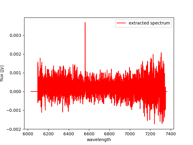
The user can also decide to visualize the extracted spectrum without saving it as a new FITS file. In that case he/she should make use of the -p option:
(megara) $ megaratools-extract_spectrum -s test/final_rss.fits \
           -t test/regions.fibers -c 2 -g Region2 -p
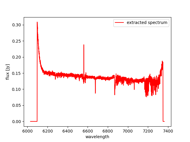
One of the uses of this tool is to extract the spectrum of the
(flux-calibrated) final_rss.fits of a standard star processed with
MegaraLcbImage to verify that it matches the corresponding tabulated
spectrum. This extraction can be done using the fiber_ids.txt file
that it is stored in the *_results/ directory generated by the MEGARA
DRP when running this recipe. In the case the command would read (using
two single quotes for the -g option we ensure that the command selects
all rows extraction):
(megara) $ megaratools-extract_spectrum -s test/final_rss.fits \
           -t test/fiber_ids.txt -c 1 -g '' -p
Extract elliptical apertures: megaratools-extract_rings
This tool (also part of megara-tools) is similar to the previous one but allows to automatically extract spectra of elliptical rings or arbitrary size, orientation and ellipticity around a given position (fiber). This is particularly useful of the analysis the radial variation of properties derived from RSS data when the signal-to-noise ratio does not allow to carry out a spaxel-by-spaxel analysis. The options for this command are:
(megara) $ megaratools-extract_rings -h
The command creates an RSS file with the same wavelength calibration
solution as the input RSS file but a number of columns equal to the
number of rings extracted (as set by the -n option). Besides, this
command when run with the verbose option (-v) on it also outputs the
main parameters of the rings extracted: average surface brightness at
the central wavelength (in Jy/spx or Jy/arcsec2 if the -b
option is set) and area. Below, we show an example of how this command
is run and of the output it creates in verbose mode.
(megara) $ megaratools-extract_rings -r test/final_rss.fits -c 311 \
           -b -w 0.6 -n 5 -s test/rings.fits -e 0.8 -pa 0. -v
Note that this tool can be also used to add the fluxes within (complete)
elliptical apertures, not only rings by using the -a option. The
resulting RSS can be used to extract the spectra of each ring/aperture
by combining its use with the megaratools-extract_spectrum tool
described in Section Extract spectrum: megaratools-extract_spectrum.
Examples of that use are:
(megara) $ megaratools-extract_spectrum -s test/final_rss.fits \
           -t test/rings.dat -c 1 -g 1 -o test/ring1.fits
(megara) $ megaratools-extract_spectrum -s test/final_rss.fits \
           -t test/rings.dat -c 1 -g 2 -o test/ring2.fits
where the test/rings.dat file is simply a list of integer numbers.
Plot spectrum: megaratools-plot_spectrum
This tool allows to plot a 1D MEGARA spectrum. It also allows to combine
the spectrum plotted with a tabulated spectrum (e.g. that from a
standard star) and a list of spectral lines. The options that can be
used for the megaratools-plot_spectrum tool are:
(megara) $ megaratools-plot_spectrum -h
Below we show an example of its use and the resulting plot (Figure 19).
(megara) $ megaratools-plot_spectrum -s test/spectrum.fits \
           -t test/mbd33d2642.dat -p -T 'BD+33 2642 spectrum' \
           -L1 6000 -L2 7500 -F1 2E-14 -F2 2E-13 -c test/bright_lines.dat
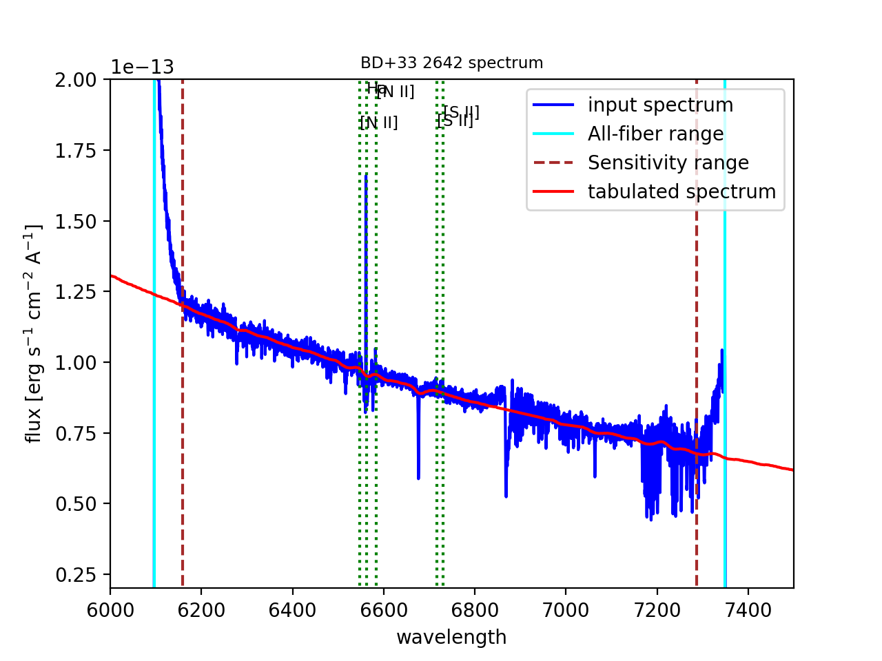
Figure 19: Result of the megaratools-plot_spectrum of standard star BD+33 2642 along with the CALSPEC tabulated spectrum and a series of spectral lines at the recession velocity of the source.
The tabulated spectrum is assumed to be in AB magnitudes and the file with a catalogue of spectral lines must have the following format:
(megara) $ cat test/bright_lines.dat
Along with the input spectrum, megaratools-plot_spectrum also shows
(see Figure 19) the wavelength limits corresponding to the spectral
range that is common to all fibers (cyan lines) and that where the
computation (smoothing) of the sensitivity curve yields a reliable flux
calibration (dashed red lines). In that regard, it is also worth noting
that this tool can be also used to plot efficiency curves generated by
the LcbStdStar recipe (e.g. master_sensitivity.fits), as shown in
Figure 14, both in their nominal units (electrons/Jy) or in relative
efficiency (when the option -e is used) assuming 80% pupil losses and
80% telescope efficiency relative to its effective area.
Diffuse light determination: megaratools-diffuse_light
In some MEGARA observations taken under bright moon conditions during 2018 and 2019 some reflected moonlight did manage to reach the spectrograph camera and the detector. This diffuse light appeared as a low-frequency pattern that could amount from just a few to tens of counts (see top-left panel of Figure 20). This tool fits this pattern using information from the region of the CCD that is not illuminated by the fibers below and above the pseudo-slit and in between the boxes that constitute it. Figure 21 shows the result of the fit of an average of 50 columns to a 4th-order polynomial to the flux of regions illuminated by diffuse light alone.
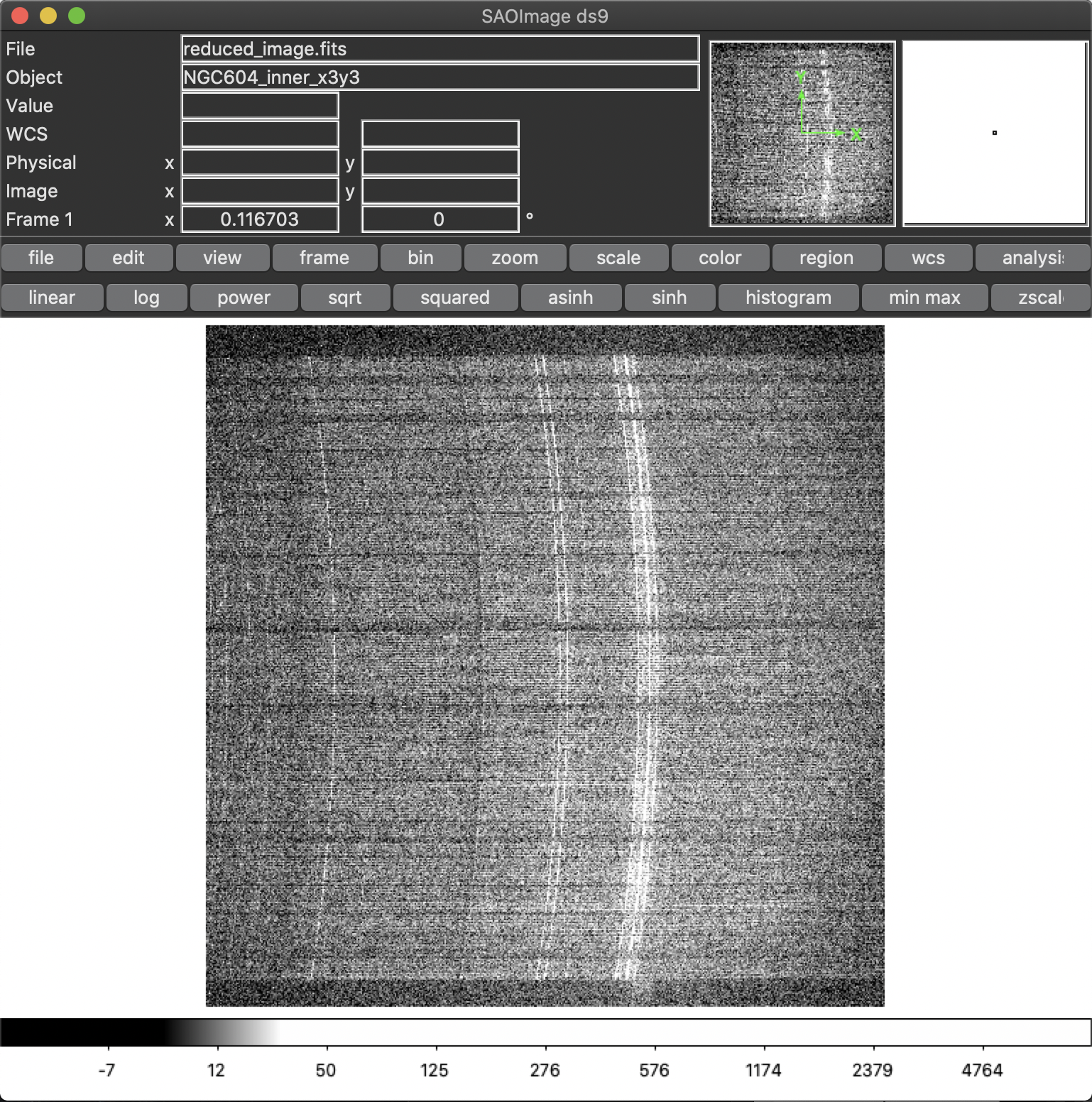
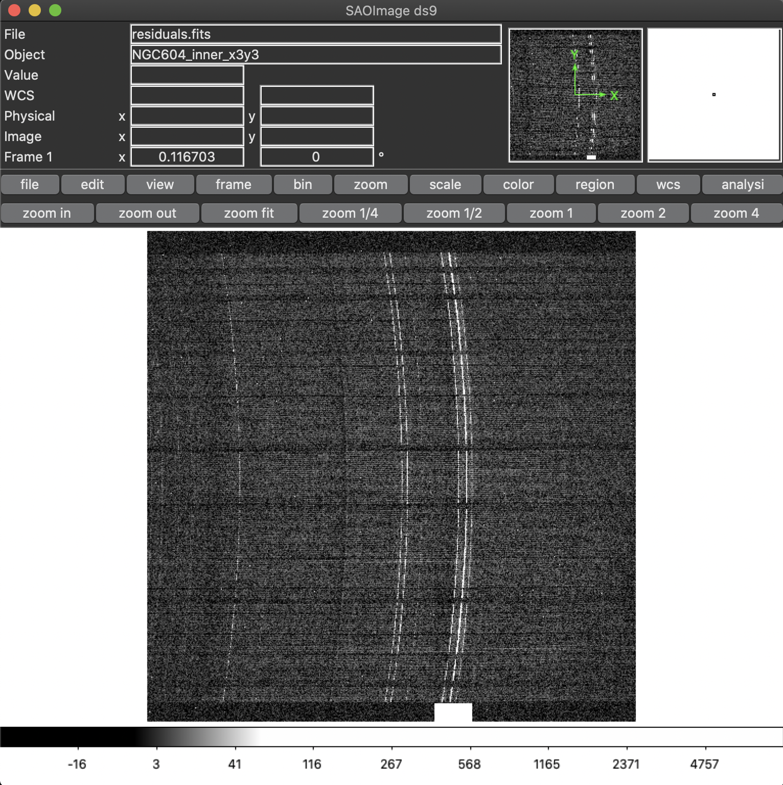
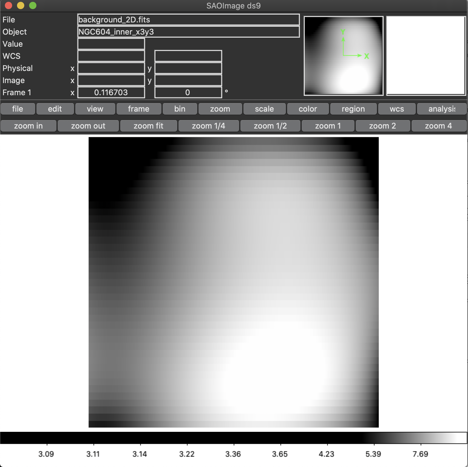
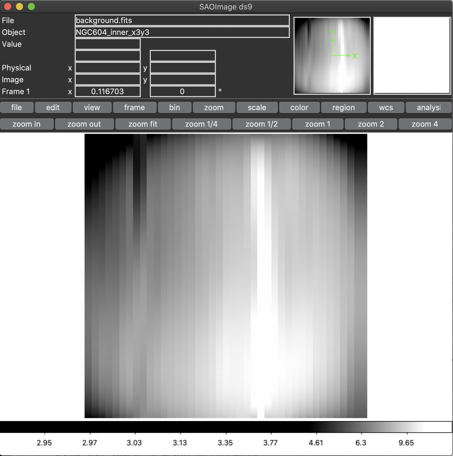
Figure 20: Example of an image with diffuse light contamination (top-left panel). The residuals after the best fit in 2D is performed is shown in the top-right panel. Low-frequency background models obtained by fitting only columns (left) and in 2D (columns first, then columns) (right) are in the bottom panels.
Below we show how this tool is executed and some basic information on its different options.
(megara) $ megaratools-diffuse_light -h
Most of these options are related to the different fitting parameters
used. Note that the input image should be the reduced_image.fits image
generated by, among others, the MegaraLcbImage and MegaraMosImage
recipes, that is place in the corresponding \*_work/ directory. This
cannot be run on raw images as those have different bias levels and
gains for its two amplifiers. A master-traces file and the offset
between them and the position of the fibers in the contaminated image
should be provided as well (options -t and -s, respectively).
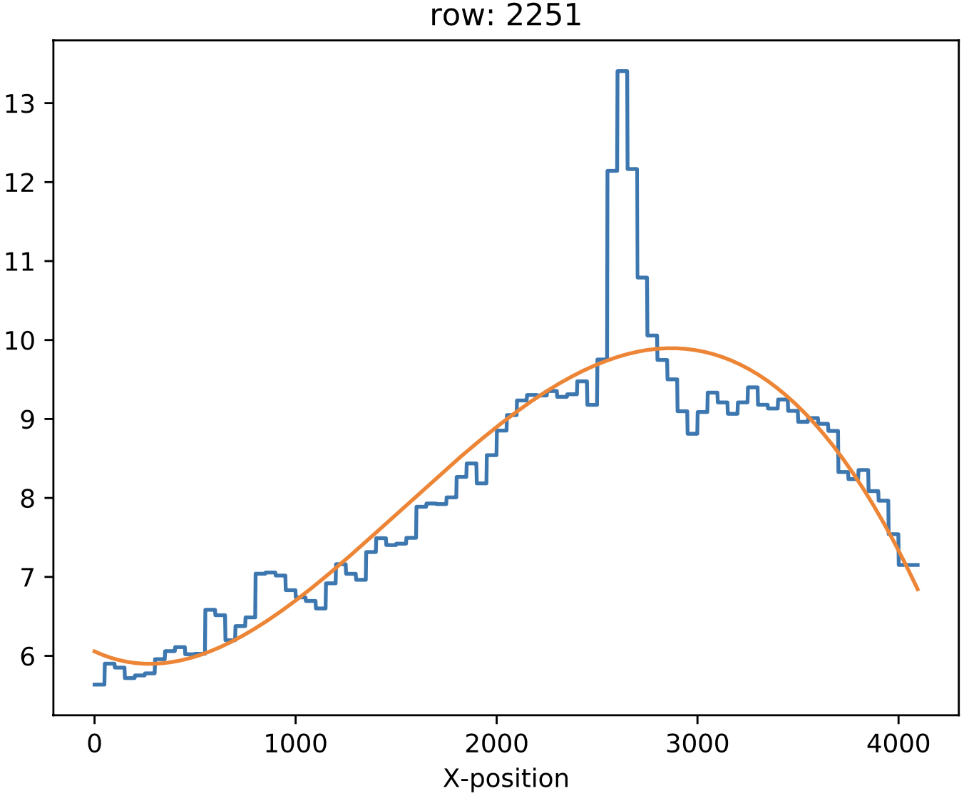
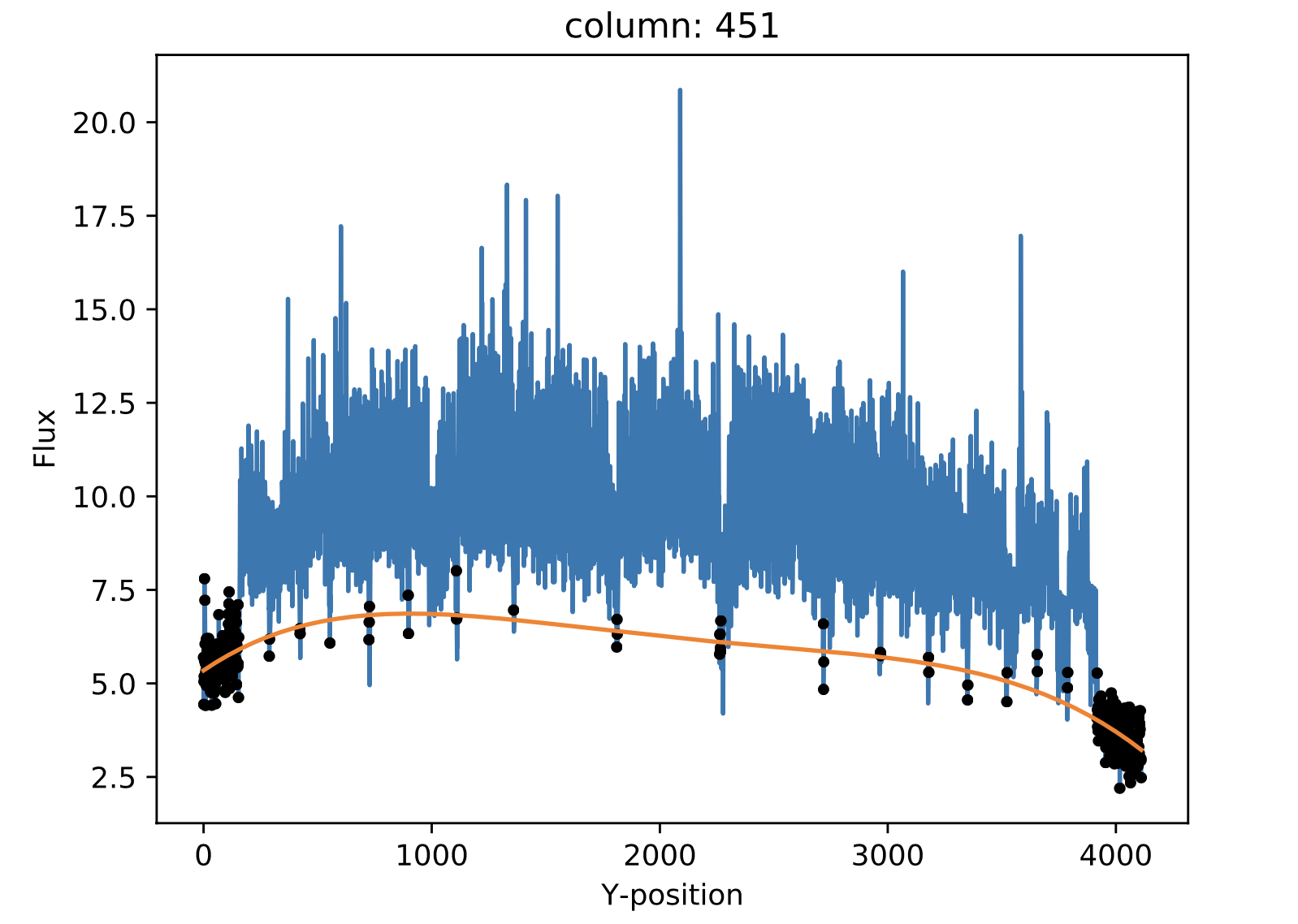
Figure 21: Fit to the sum of 50 columns (left) and 50 rows (right) for a reduced_image.fits contaminated by diffuse light. The 2D fit ensures that potential bright lines (peak in the right-panel profile) do not significantly affect the modeling results. Black points correspond to those pixels used to perform this fit. A fourth-order polynomial was used in these fits.
Option -e (defined in pixels) allows to exclude a specific region from
the fit (white rectangle in top-right panel of Figure 20). This is
particularly useful from some very early observations in the red (LR-R,
MR-R, MR-RI) in which light from the pseudo-slit mechanism LED was
adding some diffuse light just below the position of the spectra on the
CCD but not the under the light from the fibers itself, making this
region not useful to fit any low-frequency pattern present throughout
the entire CCD. An example of the use of this tool follows:
(megara) $ megaratools-diffuse_light -i test/reduced_image.fits \
  -o test/background_2D.fits -r test/residuals_2D.fits \
  -t test/master_traces.json -s 1.2 -p test/plots_2D.pdf \
  -e 2407 2720 0 154 -2D
The result of this command is a low-frequency background image (the one
set by the -o option). See the bottom panels of Figure 20 in this
regard, for the best fit along columns only (left panel) and fitting the
result also along rows (right panel). In order to remove this image
during the data processing with the DRP, both the MegaraLcbImage and
MegaraMosImage count with a requirement called diffuse_light_image
that should be set to the image resulting from this tool. That image
should be placed under the data/* directory where the megaradrp is
being run. This requirement is added in the development versions of the
megaradrp or in Python package versions released after July
1st 2020 (numina and megaradrp versions 0.22+ and 0.10+,
respectively). The user can find more info on the set of requirements of
these tasks by doing:
(megara) $ numina show-recipes -m MegaraLcbImage
This tool also generates a clean image that, although of no use within
the megaradrp, can be used to verify the quality of the low-frequency
background modeling performed (see bottom panel of Figure 20).
Output background images generated by megaratools-diffuse_light have
keyword NUM-DFL added to their headers.
Analysis of a 1D emission-line spectrum: megaratools-analyze_spectrum
There are multiple tools that perform the analysis of spectral of
astronomical sources, both the stellar continuum and emission lines
(pPXF, Steckmap, Fit3D, FADO, to name a few). However, most of these
software tools do not work right away on data from a new instrument,
although many started from the need of analyzing data from a specific
spectrograph and survey, such as SAURON (pPXF) or PPaK/CALIFA (Fit3D).
In the case of MEGARA three different tools are used, one that is based
on pPXF (see e.g. Dullo et al.
2019;
not yet public) and two that are designed for the analysis of single
emission lines on extracted 1D (megaratools-analyze_spectrum, below)
and RSS 2D MEGARA spectra (megaratools-analyze_rss, Section 6.8).
The megaratools-analyze_spectrum tool allows to determine all
parameters of a specific emission lines by fitting different functions
(linear continuum plus a modelled single gaussian, double gaussian or
Gauss-Hermite polynomials to a single emission line) within a given
spectral range. As this tool is used on extracted 1D spectrum, the
output is given on the screen and no output file is created. This tool
is executed by doing:
(megara) $ megaratools-analyze_spectrum -h
Some of the options of this task are common to the ones in
megaratools_plot_spectrum, including the possibility of adding a tabulated
spectrum (-t) or catalog of spectral lines (-c), defining the redshift
of the source (-z), creating an output PDF (-o) with or without legend
(-n). Here we show an example of its usage:
(megara) $ megaratools-analyze_spectrum \
  -s test/spectrum.fits \
  -f 2 -w 6563 -LW1 6552 -LW2 6570 -CW1 6400 -CW2 6710 \
  -ECW1 6545 -ECW2 6588 -PW1 6350 -PW2 6800 -f 2 \
  -c test/bright_lines.dat -p -k -z "-0.00025" -S2 " -0.2"
Note that setting values to -LW1, -LW2, -CW1, -CW2, -PW1,
-PW2 is mandatory. The tool, based on some of the options introduced,
determines an initial set of fitting parameters. If the -k option is set,
the initial guess on the line peak is taken from the maximum value (after the
best-fitting continuum is removed) within the specified fitting range. For the
initial guesses on the 1st and 2nd-order moments we take the
position of that maximum and some factor (~1-1.2, depending on the model
function; see below) of the instrumental FWHM. The models considered to date
are:
Gauss-Hermite polynomials (
-f 0)Single gaussian (
-f 1)Two gaussians (
-f 2)
In the case of the model with two gaussians one can scale the initial guess on the peak intensity of the second gaussian relative to the first one. This is particularly useful when underlying absorption is present in the spectral range of the fit (see Figure 22). After executing this command, it prints in the screen both the input and output (best-fitting) parameters. The content of this output also depends on the type of model function chosen to fit the emission line. The output of the example above would be the following:
FITTING CONTINUUM:
Input(slope,yord):   0.000E+00  9.724E-14
Output(slope,yord): -5.336E-17  4.468E-13
Best-fitting chisqr continuum:  7.321E-27
BASIC NUMBERS:
(mean,rms,lpk,pk,S/N) 9.682864107165422e-14 2.9143067925725397e-15 6561.03 1.658473599169167e-13 56.907996213575935
FITTING METHOD: DOUBLE GAUSSIAN
Input(i1,l1,sig1,i2,l2,sig2):   6.212E-14 6561.03  0.47 -1.380E-15 6561.03  0.93
Flux1 from model:  8.224E-14+/- 9.845E-15
Flux2 from model: -1.117E-13+/- 9.573E-15
Output(i1,l1,sig1,i2,l2,sig2):  8.308E-14 6561.11  0.39 -1.263E-14 6561.31  3.63
Flux & EW from data:  -2.844E-14+/- 9.690E-15 -0.29+/- 0.10
Flux & EW from model: -2.949E-14+/- 9.689E-15 -0.30+/- 0.10
Best-fitting chisqr:  2.279E-28
Note that the term from data refers to the sum of the flux above the
continuum within the spectral range used to fit the line profile, while
the term from model refers to the analytic integral of the model.
Besides, megaratools-analyze_spectrum displays a plot (similar to the
ones shown in Figure 22) that includes:
The input spectrum in the range set by options
-PW``1 and ``-PW2(blue line)Vertical lines of the different spectral ranges of interest, including the range covered by all fibers (cyan line) and with precise flux calibration in the original RSS frame (dashed red line), the range for fitting the continuum (dashed grey lines) and that where the line fit is performed (solid gray line).
Best-fitting continuum (solid red line).
Best-fitting line plus continuum (solid orange line).
The user should check the ranges chosen and then kill the graphical terminal for the code to start running.
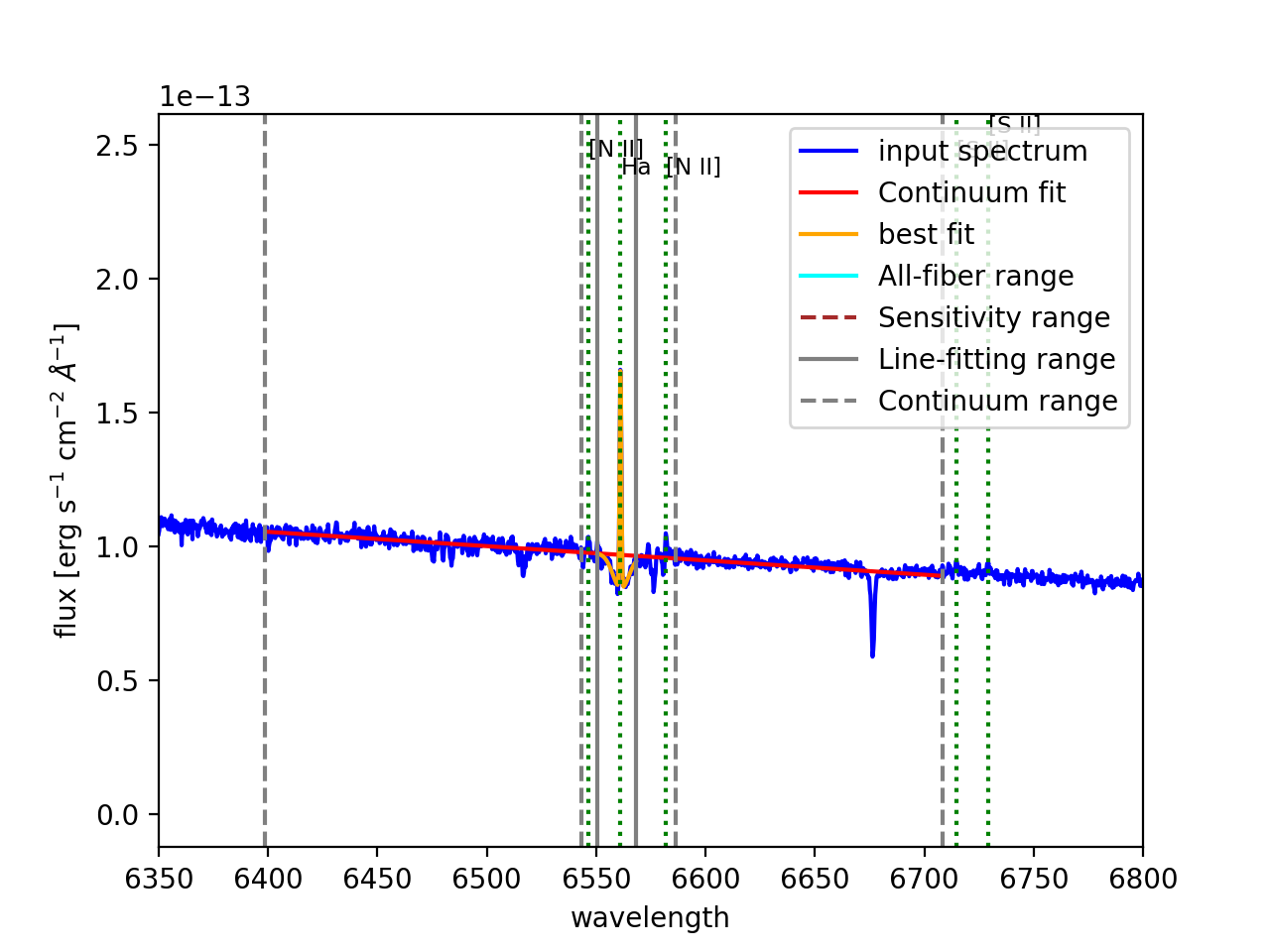
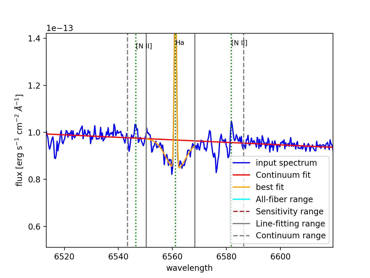
Figure 22: Two different views of the plot generated by megaratools-analyze_spectrum for the example given in the text. In this case the line fitted is \({\rm H}\alpha\) and the method used was a double gaussian, where the intensity of the secondary gaussian was set to negative 20% of the intensity of the primary one to model the underlying absorption in this (Balmer) line.
Analysis of a 2D RSS emission-line spectrum: megaratools-analyze_rss
Based on the fitting procedure of megaratools-analyze_spectrum tool we
also developed a tool that is able to do the same spectral analysis in
MEGARA RSS files. This is particularly useful for creating maps of
derived properties (fluxes, line-of-sight radial velocity and velocity
dispersion and higher-order momenta) from the analysis of LCB RSS final
data (final_rss.fits or reduced_rss.fits files created by the
MegaraLcbImage recipe).
The tool is called megaratools-analyze_rss and it is executed by
doing:
(megara) $ megaratools-analyze_rss -h
Although the spectral ranges and model function set by the options of
the parameter are common to all fibers, option -S allows to set a
minimum signal-to-noise ratio for the peak intensity below which no fit
is attempted. The verbose mode allows to print to screen the same output
results as those shown by default by the megaratools-analyze_spectrum
tool but for each individual fiber fulfilling the minimum S/N criteria
imposed.
The rest of the options are identical to the ones described for the
megaratools-analysis_spectrum tool. The main difference comes from the
output products. While in the case of the megaratools-analysis_spectrum
tool only printed output is produced, this tool generates an RSS FITS file of
products that has the same number of rows as the input RSS (623 or 644) but
only 29 columns, one per derived property, including the majority of the model
best-fitting parameters. The properties included in columns 0 to 28 of the
output RSS and their meaning are listed above as part of the online help
information provided by the tool (-h option). The output also includes a
PDF file with the graphical result of all fibers that were fit (plots with the
original spectra of fibers with S/N below the number given in option -S are
also included) and an ascii file listing the ids of the fibers that matched our
minimum S/N requirement. This file is useful as it can be used (in combination
with megaratools-extract_spectrum) to generate a high-S/N emission-line
spectrum of our target. Figure 23 shows the plots generated for two
specific fibers and two different spectral lines using the instructions given
later in this section.
Below we provide two examples of the execution of the
megaratools-analyzed_rss tool for two different spectral lines in the
same spectral setup: \({\rm H}\alpha\) and \([{\rm NII}]\lambda
6584\). Right after each of these
commands is executed, the program shows a plot of the integrated
spectrum (all fiber spectra added up) with all relevant spectral ranges
clearly identified with vertical lines. The RSS product files generated
by these two instructions will be later used to compute an RSS file that
can be used to create a line-ratio map.
(megara) $ megaratools-analyze_rss \
  -s test/final_rss.fits -f 2 \
  -w 6563 -LW1 6552 -LW2 6570 -CW1 6400 -CW2 6710 \
  -ECW1 6545. -ECW2 6588 -PW1 6350 -PW2 6800 -f 2 -k \
  -z "-0.00025" -S2 " -0.2" -S 5 \
  -o test/analyze_rss_Halpha.pdf \
  -O test/analyze_rss_Halpha.fits \
  -of test/analyze_rss_Halpha.fibers

(megara) $ megaratools-analyze_rss \
  -s test/final_rss.fits -f 2 \
  -w 6584 -LW1 6580 -LW2 6587 -CW1 6400 -CW2 6710 \
  -ECW1 6545. -ECW2 6588 -PW1 6350 -PW2 6800 -f 1 -k \
  -z "-0.00025" -S 5 \
  -o test/analyze_rss_N2.pdf \
  -O test/analyze_rss_N2.fits \
  -of test/analyze_rss_N2.fibers
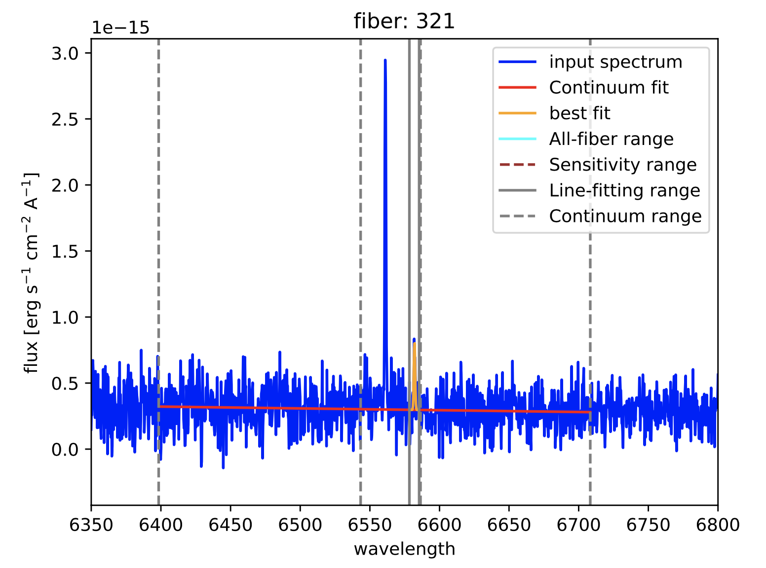
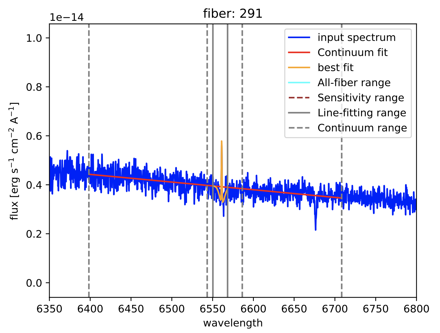
Figure 23: Results of the fitting of \({\rm H}\alpha\) (left panel) and \([{\rm NII}]\lambda6584\) (right panel) spectral lines for fibers 291 and 321, respectively. As for the graphical output of megaratools-analyze_spectrum, the input spectrum is shown in blue, the range used for the fitting the continuum is bracketed between dashed grey lines, the range for fitting the line in between solid grey lines, the best-fitting continuum is shown as a solid red line and the best-fitting line plus continuum is in orange.
RSS arithmetics: megaratools-rss_arith
The tool megaratools-rss_arith described here allows to perform basic
computations (Python basic arithmetic and numpy numerical operations)
on RSS files. The online help output is shown below.
(megara) $ megaratools-rss_arith -h
The input of this tool is a text file with the list of images involved in the operation (all of the same size):
(megara) $ cat test/images.txt
The output is always an RSS file with one single column and the same number of rows as the input images. The philosophy behind of this tool is rather similar to that of the imexpr command in IRAF.
The tool can be used for multiple purposes using any of the numpy
array operations. Below we show examples of some potential usages of
megaratools-rss_arith. For example:
(megara) $ megaratools-rss_arith \
  test/images.txt \
  -e 'np.log10(ima1[:,6]/ima2[:,22])' \
  -o test/logN2_over_Ha_rss.fits
This instruction includes the options required to create a line-ratio RSS (in
log10 scale) from two RSS FITS files created by the megaratools-analyze_rss
tool for the \({\rm H}\alpha\) and \([{\rm NII}\lambda6584]\) lines.
Note that, given that we are using only the flux of the emission component of
\({\rm H}\alpha\), we use channel #22, which corresponds to the line flux
of only the primary gaussian (see description of tool
megaratools-analyze_rss in Section 6.8), for \({\rm H}\alpha\) and
channel #6 for \([{\rm NII}\lambda6584]\).
Other examples are:
(megara) $ megaratools-rss_arith test/images.txt \
  -e '(np.mean(ima3[:,1000:2000],axis=1))' \
  -o test/mean_1000_2000.fits

(megara) $ megaratools-rss_arith test/images.txt \
  -e '(np.mean(ima3[:,2000:3000],axis=1))' \
  -o test/mean_2000_3000.fits
In these cases, we compute the mean of all the flux from spectral pixels 1000 to 2000 (top) and 2000 to 3000 (bottom) to create two new separated RSS files. We can now create a spectral-index-like RSS image by running:
(megara) $ megaratools-rss_arith test/images2.txt \
  -e 'ima4[:,0]/ima5[:,0]' \
  -o test/index.fits
The user should bear in mind that test/images2.txt now includes two
additional rows with the names of the images created above:
test/mean_1000_2000.fits and test/mean_2000_3000.fits. Note that
although the images listed in the test/images2.txt file would have
different dimensions we would not get any error because (1) they have
the same number of rows (623 in this case) and (2) images of different
dimensions are not combined in the same execution of
megaratoos-rss_arith. We show in Figure 24 the resulting
test/index.fits RSS image using the megaradrp.visualization tool
described in Section 6.1. This figure was obtained using the command:
(megara) $ python -m megaradrp.visualization test/index.fits \
  -c 0 --min-cut 0.8 --max-cut 1.2
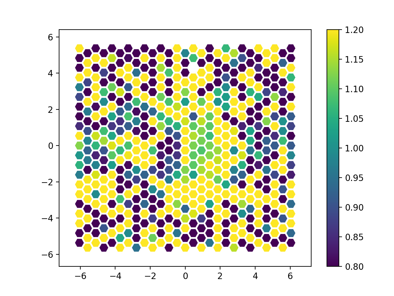
Figure 24: Ratio between the mean_1000_2000.fits and
mean_2000_3000.fits images generated with megaratools-rss_arith.
Note that the spectral range explored by this spectral-index image is rather small, which leads to a very small dynamic range. Nevertheless, most of the spaxels showing bright emission from the source reveal a relatively blue color as expected for the spectral type of this spectrophotometric standard star.
The user should be also aware when using this tool that any operation involving a logarithmic or intensity ratios might lead to some warnings. These tools should properly handle (and create when necessary) NaN values but we cannot guarantee that any other software to be run on these products will have no issues using these data.
We note that megaratools-rss_arith can be also used on extracted (1D)
spectra created with the megaratools-extract_spectrum tool described
in Section 6.3. The instruction to use it on extracted spectra would be
something like the following:
(megara) $ megaratools-rss_arith test/list_1D \
  -e '2.0*ima1+ima2' \
  -o test/output_1D.fits
where list_1D should be a text ascii file with the (in this case, two)
extracted spectra on which the numerical operation is to be performed
(similar to the test/images.txt file quoted above for RSS files) and
output_1D.fits would be the output 1D spectrum. This output file is
fully compatible with our megaratools-plot_spectrum or
megaratools-analyze_spectrum tools.
Megaratools-hypercube
Some observations with the MEGARA LCB might require of acquiring
multiple points to mosaic an extended astrophysical object. In order to
combine the information from all the different RSS files generated by
the DRP from each of the individual observations we have developed a
code based on the megaradrp-cube tool but that is able to handle a
series of RSS files placed at different adjacent positions in the sky
combined them all together to create a single large cube. This tool is
called megaratools-hypercube and its online help can be obtained by
doing:
(megara) $ megaratools-hypercube -h
Although this tool determines the position on the sky based on the image WCS solution, it also allows to apply additional RA & Dec offsets to each of the individual generated cube sections (one from input RSS frame). Besides, one can also shift and scale the flux levels of each of the cube sections to take into account possible non-photometric conditions during the observation. These corrections are introduced as part of the input file where the list of RSS images to combine are included. An example of such a file is given below:
(megara) $ cat test/list_hypercube
The first column is the RSS filename, columns 2 and 3 correspond to the offsets (in arcsec) of the different pointings, column 4 allows to introduce offsets to the flux levels measured in the corresponding pointing and column 5 is the scaling factor to be applied to the flux of each pointing. The example listed above would be the one to be used if the astrometry and flux calibration of all RSS files is perfect.
An example of how the tool should be run would be the following:
(megara) $ megaratools-hypercube test/list_hypercube \
  -l -o test/cube.fits -p 0.4 -m linear \
  --wcs-pa-from-header -trim -hyp -helio
In this case the pixel size of the cube.fits output file would be 0.4
arcsec/pixel, the cube would be generated using linear interpolation, 2
two rows and 1 bottom row, 1 left and right columns would be removed
from each cube before they are combined together. The best number of
rows and columns to be removed depends on the pixel size, so it can be
modified by using the -trimn option. Besides,
megaradrp-tools_hypercube allows to put all (topocentric) wavelength
calibrations to a common barycenter wavelength calibration.
The use can also use this tool to simply generate a list of cubes from
individual RSS files by removing the -hyp option.